棱柱形谐振器
目录
本页讨论棱柱形谐振器的性能(即截面尺寸在振动主方向上保持不变的谐振器)。
除非另有说明 —
- 谐振器均为圆柱形。
- 谐振器不包含螺柱或螺柱孔。
- 主振动模态为轴向。(对于直径非常大的谐振器,径向振幅可能超过轴向振幅。尽管如此,所研究的仍是轴向模态。)
- 振幅、应变和应力均沿谐振器的轴线中心线确定。
- 性能数据由有限元分析(FEA)确定。(在某些情况下,若理论值与 FEA 值无显著差异,则采用理论值。)
轴向振幅
棱柱形谐振器的轴向振幅自自由端起沿谐振器长度呈余弦分布 —
\begin{align} \label{eq:10701a} u(x) &= U_p \cos \left( \frac{\pi}{\Gamma} \, x \right) \end{align}
式中 —
| \( u \) | = 振幅分布 |
| \( x \) | = 距离,自自由端(波腹)起算 |
| \( U_p \) | = 最大(峰值)振幅 |
| \( \Gamma \) | = 谐振频率下的半波长 |
括号( )内的量以弧度为单位。振幅 \( u(x) \) 在波腹处(自由端以及此后每隔一个半波长(\( \Gamma \))处)最大。\( u(x) \) 在波节处(\( \Gamma/2 \) 以及此后每隔一个 \( \Gamma \) 处)为零。对于细线,\( \Gamma \) 就是细线半波长 \( \Gamma_{tw} \)。
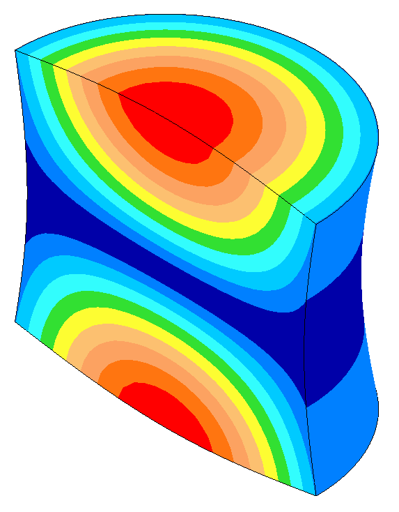
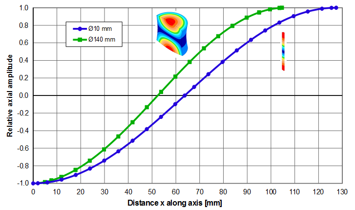
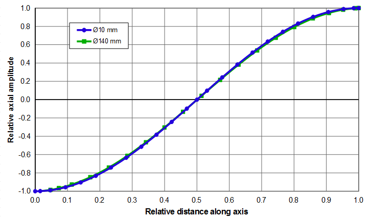
公式 \eqref{eq:10701a} 无论谐振器是细是粗都适用。图 1 中的两个 20 kHz 谐振器说明了这一点——一个为 \( \phi \)10 mm(相当细),另一个为 \( \phi \)140 mm(明显很粗)。沿每个谐振器轴线的振幅数据绘制于图 2。左图中的数据为对应实际谐振器长度的振幅分布。右图显示相同的数据,但 X 轴已对两个谐振器的半波长作了归一化——即 \( \large\frac{x}{\Gamma_{\phi 10}} \) 和 \( \large\frac{x}{\Gamma_{\phi 140}} \)。右图中的两条曲线几乎重合,表明细、粗谐振器均可用公式 \eqref{eq:10701a} 描述。
|
||||||||||
|

|
||||||||||
|
轴向应变与应力
细线仅在轴向方向上承受应变。此时轴向应变是振幅曲线的导数(斜率) —
\begin{align} \label{eq:10702a} {\epsilon}(x) &= \frac{du}{dx} \\[0.7em]%eqn_interline_spacing &= U_p \left( {\frac{\pi}{\Gamma_{tw}}} \right) \sin \left( {\frac{\pi}{\Gamma_{tw}}} \, x \right) \nonumber \end{align}
应变 \( {\epsilon}(x) \) 在波腹处(自由端以及此后每隔一个半波长(\( \Gamma_{tw} \))处)为零。\( {\epsilon}(x) \) 在波节处(\( \Gamma_{tw}/2 \) 以及此后每隔一个 \( \Gamma_{tw} \) 处)最大。
\begin{align} \label{eq:10707a} {\epsilon}_{max} &= U_p \left( {\frac{\pi}{\Gamma_{tw}}} \right) \end{align}
上述公式也可以不用半波长表示,而用频率和波速表示更为方便,其中应注意到 —
\begin{align} \label{eq:10703a} \Gamma_{tw} = \frac{c_{tw}}{2 \, f} \end{align}
式中 —
| \( c_{tw} \) | = 细线波速 = \( \sqrt{\frac{E}{\rho}} \) |
| \( f \) | = 频率 |
于是公式 \eqref{eq:10701a} 至 \eqref{eq:10707a} 变为 —
\begin{align} \label{eq:10704a} u(x) &= U_p \cos \left( {\frac{2\pi \, f}{c_{tw}}} \, x \right) \end{align}
\begin{align} \label{eq:10705a} {\epsilon}(x) &= U_p \left( {\frac{2\pi \, f}{c_{tw}}} \right) \sin \left( {\frac{2\pi \, f}{c_{tw}}} \, x \right) \end{align}
\begin{align} \label{eq:10706a} {\epsilon}_{max} &= U_p \left( {\frac{2\pi \, f}{c_{tw}}} \right) \end{align}
粗径谐振器
如上所述,无论谐振器是细是粗,沿谐振器轴线的振幅均为余弦分布(公式 \eqref{eq:10701a})。然而,应变公式 \eqref{eq:10702a} 仅在应变沿单一方向作用时适用,这对细长谐振器成立。由于以下两个效应,粗径谐振器的净应变会更高 —
- 除轴向运动外,粗径谐振器还因泊松耦合而产生横向“呼吸”运动。这会引入额外的径向和周向(环向)应变。
- 粗径谐振器的调谐长度更短(即 \( \Gamma \lt \Gamma_{tw} \)),因此给定的振幅被压缩在更短的长度内。
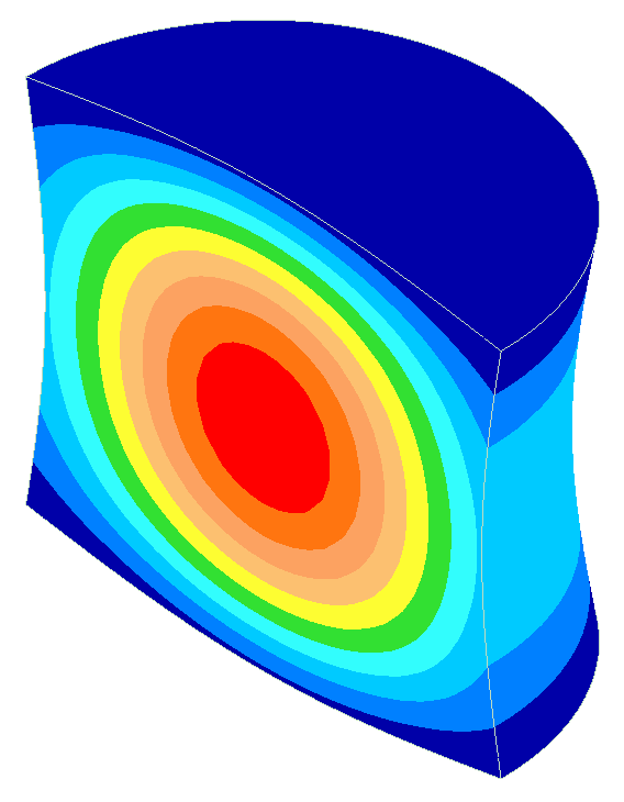
这两个效应的综合结果如图 3 和图 4 所示(20 kHz 谐振器)。\( \phi \)10 mm 谐振器相当细,其应变可由公式 \eqref{eq:10702a} 预测。而 \( \phi \)140 mm 谐振器则相当粗 —
- 其半波长比细谐振器短 18%(105 mm 对 127 mm)。
- 其峰值应变比细谐振器高 36%。
- 自由端面(波腹)处的应变不为零;而是波节处应变的 6%。这是因为自由端具有显著的径向振幅(为端面轴向中心线振幅的 5%)。
|
||||||||||
|

|
|
|
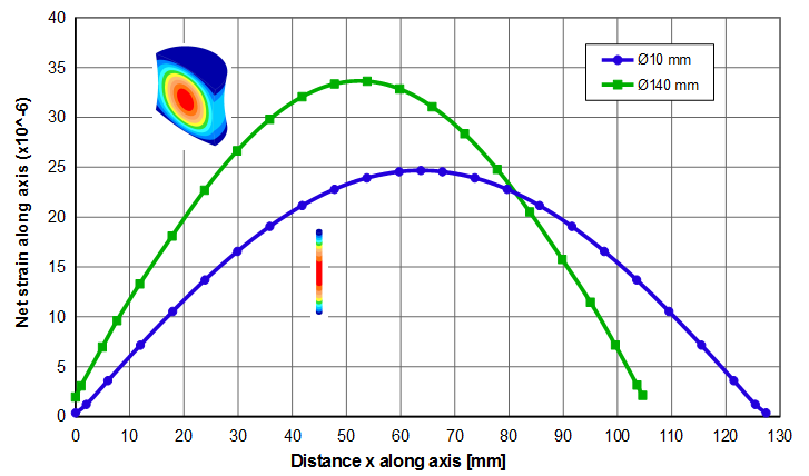
注:上图所示净应变为 von Mises 应变。von Mises 应力可由杨氏模量 \( E \) 与 von Mises 应变的乘积计算。
调谐
棱柱形谐振器的调谐取决于谐振器直径与其棱柱形半波长之比。
调谐长度
细长棱柱形谐振器的调谐长度为 —
\begin{align} \label{eq:10710a} \Gamma_{tw} = \frac{c_{tw}}{2 \, f} \end{align}
式中 —
| \( \Gamma_{tw} \) | = 细线半波长 |
| \( c_{tw} \) | = 细线波速 |
| \( f \) | = 频率 |
细线波速可由材料性能确定 —
\begin{align} \label{eq:10711a} c_{tw} &= \sqrt{\frac{E}{\rho}} \end{align}
式中 —
| \( E \) | = 弹性模量(杨氏模量) |
| \( \rho \) | = 密度 |
随着谐振器横向尺寸增大(即谐振器不再“细长”),半波长会降至细线半波长以下。从物理上看,当谐振器直径大于无限细的细线时,泊松耦合会引起径向“呼吸”。这种径向运动带来额外的动能,会使谐振器频率下降。为了维持期望的频率,必须缩短谐振器的长度。
直径更大时呼吸更为显著,谐振器必须调得更短。在最大可能的直径下,谐振器退化为一个薄平圆盘。此时呼吸就是圆盘的基频径向谐振。
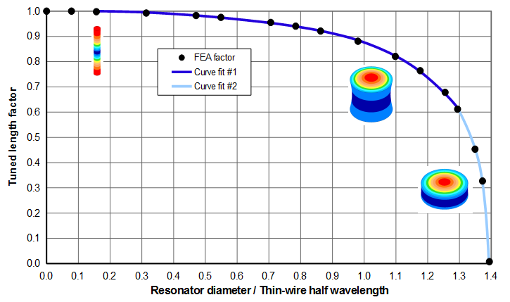
有限直径 \( D \) 下的实际调谐长度可由 \( \Gamma_{tw} \) 乘以长度因子 \( K_L \) 确定。
\begin{align} \label{eq:10712a} \Gamma = K_L \,\, \Gamma_{tw} \end{align}
式中 —
| \( \Gamma \) | = 直径 \( D \) 下的半波长 |
| \( \Gamma_{tw} \) | = 细线半波长 |
| \( K_L \) | = 调谐长度因子 |
调谐长度因子可由图 5 或图 6 确定。(图 6 是图 5 的局部放大,其横轴限制在 1.1 以内,这是大多数轴向谐振器现实可行的上限。图 6 还包含了多种声学材料典型的泊松比范围。为清晰起见,未标出各个 FEA 数据点。)图中的图像显示了圆柱的相对尺寸;颜色代表轴向振幅(平行于谐振器轴线)。
(注:两个理论近似长度因子——Rayleigh 因子 \( K_{L_R} \) 和 Mori 因子 \( K_{L_M} \)——在附录 A 中讨论。)
|
|
|
|
|
|
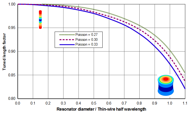
图 6 表明,调谐长度随泊松比减小而增大。事实上,若泊松比为零,则不存在泊松耦合,谐振器不会发生呼吸。此时无论谐振器直径多大,调谐长度都与细线相同。
示例 1
已知——一个 20 kHz、\( \phi \)90 mm 的圆柱形谐振器。谐振器材料的细线波速 \( c_{tw} \) 为 5100 m/sec,泊松比为 0.33。
求 — 调谐半波长 \( \Gamma \)。
- \( \Gamma_{tw} \) = 127.5 mm(公式 \eqref{eq:10710a})
- \( D/\Gamma_{tw} \) = 90.0/127.5 = 0.71
- \( K_L \) = 0.955(由图 6)
- \( \Gamma \) = 0.955 * 127.5 mm = 121.8 mm
调谐速率
由附录 B,细长棱柱形谐振器的调谐速率为 —
\begin{align} \label{eq:10715a} \varphi_{tw} &= -\frac{f}{n \, \Gamma_{tw}} \end{align}
式中 —
| \( \varphi_{tw} \) | = 细线调谐速率 [Hz/mm] |
| \( f \) | = 当前频率 [Hz] |
| \( \Gamma_{tw} \) | = 细线半波长 [mm] |
| \( n \) | = 半波数量 |
注意,负号表明调谐速率总是负值。不过,调谐速率通常以正值(绝对值)来讨论。
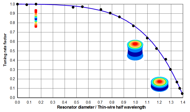
随着谐振器横向尺寸增大(即谐振器不再“细长”),调谐速率下降(即为实现给定的频率变化必须去除更多材料)。这可以通过对公式 \eqref{eq:10715a} 施加一个调谐速率因子来处理 —
\begin{align} \label{eq:10716a} \varphi &= K_T \, \varphi_{tw} \\[0.3em]%eqn_interline_spacing &= K_T \, \left( \frac{f}{L} \right) \nonumber \end{align}
注意,本节的公式仅在谐振器为棱柱形时适用。若谐振器具有增益,则不适用。
|
|
|
|
|
|
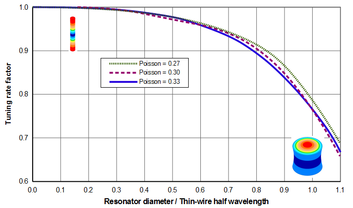
如上所述,随着横向尺寸增大(即 \( D/\Gamma_{tw} \) 增大),谐振器调得更短。似乎较短的谐振器调谐速率应当更高——即(相对于缩短后的谐振器长度)每单位长度变化应更有效地改变频率。例如,从 127 mm x \( \phi \)20 mm 的谐振器上去除 1 mm,其长度减少 0.8%;而从 105 mm x \( \phi \)140 mm 的谐振器上去除 1 mm,其长度减少 1.0%;因此按逻辑推断,105 mm 谐振器的调谐应当比 127 mm 谐振器更快(假设两者初始频率相同)。
然而,这忽略了泊松耦合引起的横向振动的影响。细长谐振器的横向振动相对较小,因此动能主要来自纵向振动。随着横向尺寸增大,谐振器的横向振动也随之增大,横向动能相应增加。当从端面对谐振器进行调谐时,横向动能相对不受影响,尤其是因为横向动能主要储存在波节区域。因此,为使“粗径”谐振器的总体动能改变与细谐振器相同的比例,必须从其端面去除更多的材料。(这正是 Rayleigh 最初用于其调谐长度修正的推理。)因此,“粗径”谐振器的调谐比细谐振器慢。对于上述例子,127 mm x \( \phi \)20 mm 谐振器的调谐速率为 157 Hz/mm,而 105 mm x \( \phi \)140 mm 谐振器的调谐速率为 100 Hz/mm(慢 36%)。
有趣的是,图 8 表明当泊松比在 0.27 至 0.33 之间时,调谐速率相对不受泊松比影响。然而,当泊松比显著偏离该范围时情况则不然。例如,若泊松比为零,则不存在呼吸,调谐速率就是细线的调谐速率,与谐振器直径无关。
示例 2
已知——一个 \( \phi \)90 mm x 半波的圆柱形谐振器。长度为 124.8 mm,对应频率为 19500 Hz。谐振器材料的细线波速 \( c_{tw} \) 为 5100 m/sec,泊松比为 0.33。
求 — 调谐速率 \( \varphi \) 及预期的最终长度。
- \( \Gamma_{tw} \) = 130.8 mm @ 19500 Hz(公式 \eqref{eq:10710a})
- \( D/\Gamma_{tw} \) = 90.0 / 130.8 = 0.688
- \( K_T \) = 0.94(由图 8)
- \( f/\Gamma_{tw} \) = 19500 Hz / 130.8 mm = 149 Hz/mm(细线调谐速率)
- \( \varphi \) = 0.94 * 149 Hz/mm = 140 Hz/mm
换能器的影响
接入换能器会将叠堆从半波系统变为全波系统,并影响调谐速率。其确切影响无法预测;但它取决于谐振器相对于换能器的储能大小。若谐振器与换能器储能相近,则调谐速率接近全波棱柱形谐振器(即公式 \eqref{eq:10716a} 中 \( n = 2 \))。然而,若谐振器储能相对较高(例如大直径钢谐振器),则换能器影响很小,调谐速率仅略低于单独的半波谐振器(公式 \eqref{eq:10716a} 取 \( n = 1 \),或查图 7、图 8)。
相对振幅
当谐振器沿轴向膨胀和收缩时,泊松耦合使谐振器产生横向呼吸。这种呼吸并不均匀,而是在应变最大处(即波节处)占主导。这导致谐振器端面上轴向振幅分布不均匀。参见进一步说明。
端面轴向振幅
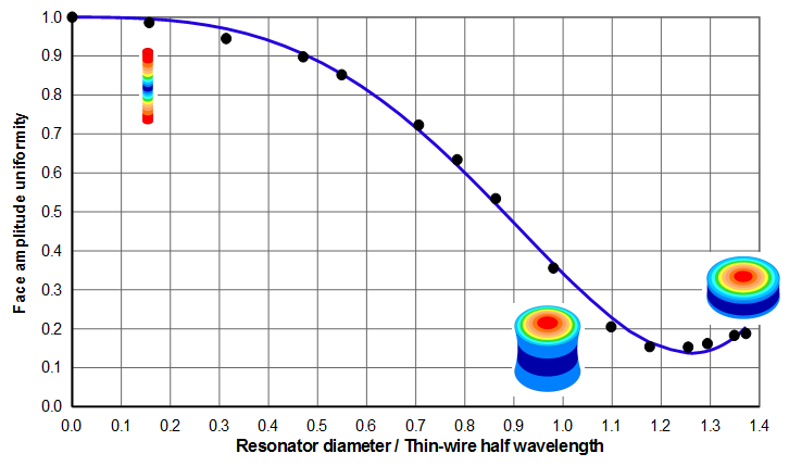
图 9 和图 10 显示端面振幅的均匀性。(参见均匀性计算(基础)。)注意,图 10 只是图 9 的局部放大,其横轴限制在 1.1 以内。
|
|
|
|
|
|
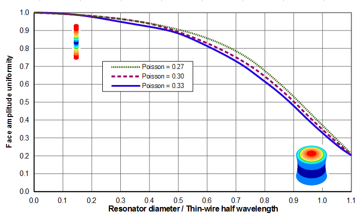
图 10 表明,随着泊松比减小,端面振幅均匀性有所改善。最大的改善出现在 \( D/\Gamma_{tw} \) 约为 0.7 时。当泊松比从 0.33 降至 0.27 时,均匀性从 0.72 提高到 0.78(改善 8%)。
曲线拟合
对图 9 和图 10 中泊松比为 0.33 的数据进行的多项式曲线拟合为 —
\begin{align} \label{eq:10718a} U = 1 - 0.0809 \, X^2 - 0.5688 \, X^3 - 0.6565 \, X^4 + 0.6481 \, X^5 \end{align}
式中 —
| \( U \) | = 端面轴向振幅均匀性 |
| \( X \) | = 圆柱直径 / 细线半波长 |
| = \( D/\Gamma_{tw} \) |
径向振幅
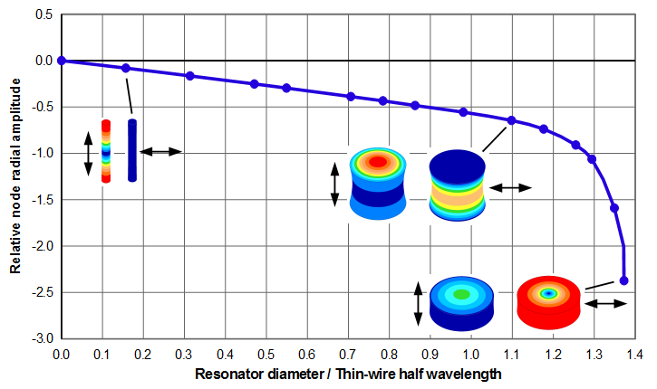
对于下列各图 —
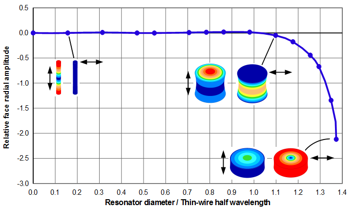
- 径向振幅均相对于谐振器端面中心处的轴向振幅。
- 作为参照,每对图像中的左图显示轴向振幅分布。
- 箭头指示相应颜色的振动方向。
- 颜色的选取使红色代表每对图像中的最大振幅。
- 径向振幅绘为负值。这仅表示径向振幅与轴向振幅反相(即谐振器沿轴向膨胀时端面沿径向收缩,反之亦然)。
波节处径向振幅
图 11 显示波节处的径向振幅。
|
|
|
端面径向振幅
图 12 显示端面边缘处的径向振幅。在谐振器直径等于细线半波长(\( \Gamma_{tw} \))之前,径向振幅基本为零;此后径向振幅迅速增大。事实上,随着圆柱形状趋近圆盘,端面径向振幅逐渐接近波节处径向振幅,这可以从最右侧谐振器图像的颜色中看出。
|
|
|
附录 A. 粗径圆柱棱柱形谐振器的调谐长度
(Rayleigh 近似与 Mori 近似)
对于以纵向模态振动的细长棱柱形谐振器,压力波的半波长为 —
\begin{align} \label{eq:10750a} \Gamma_{tw} = \frac{c_{tw}}{2 \, f} \end{align}
式中 —
| \( \Gamma_{tw} \) | = 细线半波长 |
| \( c_{tw} \) | = 纵向细线波速 |
| \( f \) | = 频率 |
纵向细线波速可由材料性能确定 —
\begin{align} \label{eq:10751a} c_{tw} &= \sqrt{\frac{E}{\rho}} \end{align}
式中 —
| \( E \) | = 弹性模量(杨氏模量) |
| \( \rho \) | = 密度 |
随着谐振器横向尺寸增大(即谐振器不再“细长”),半波长会降至细线半波长以下。从物理上看,当谐振器直径大于无限细的细线时,泊松耦合会引起径向“呼吸”。这带来额外的动能,会使谐振器频率下降。为了维持期望的频率,必须缩短谐振器的长度。
直径更大时呼吸更为显著,谐振器必须调得更短。在最大可能的直径下,谐振器退化为一个薄平圆盘。此时呼吸就是圆盘的基频径向谐振。
Rayleigh 近似
Rayleigh (1)(第 1 卷,第 251–252 页)首先提出了一个近似考虑棱柱圆柱这一现象的公式。
\begin{align} \label{eq:10752a} \Gamma = K_{L_R} \,\, \Gamma_{tw} \end{align}
式中 —
| \( \Gamma \) | = 圆柱直径 \( D \) 下的半波长 |
| \( \Gamma_{tw} \) | = 细线半波长 |
| \( K_{L_R} \) | = Rayleigh 长度因子 |
\begin{align} \label{eq:10753a} K_{L_R} = 1 - \small\frac{1}{8} \normalsize \left(\pi \, \nu \, \frac{D}{\Gamma_{tw}} \right)^2 \end{align}
式中 —
| \( D \) | = 谐振器直径 |
| \( \nu \) | = 泊松比 |
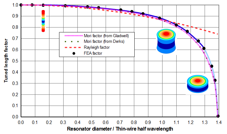
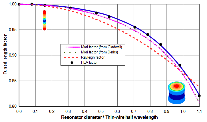
注意,\( K_{L_R} \) 取决于谐振器直径(\( D \))与细线半波长(\( \Gamma_{tw} \))之比。当 \( D = 0 \) 时,\( K_{L_R} = 1 \),于是 \( \Gamma = \Gamma_{tw}\)(即精确解)。然而,随着谐振器直径增大,Rayleigh 近似先是低估、然后又高估调谐长度(图 A1 和图 A2,典型声学材料)。
Mori 近似
Mori (1) 改进了 Rayleigh 的工作,提出的公式对细线以及大直径下的径向振动圆盘都是正确的。中间直径处的结果则用一种称为“表观弹性”的方法近似。
\begin{align} \label{eq:10754a} \Gamma = K_{L_M} \,\, \Gamma_{tw} \end{align}
式中 —
| \( \Gamma \) | = 圆柱直径 \( D \) 下的半波长 |
| \( \Gamma_{tw} \) | = 细线半波长 |
| \( K_{L_M} \) | = Mori 长度因子 |
\begin{align} \label{eq:10755a} K_{L_M} = \left[ \frac{1 - B_1 \, \psi}{1 - B_2 \, \psi} \right]^{1/2} \end{align}
式中 —
| \( B_1 \) | = \( 1 - \nu^2 \) |
| \( B_2 \) | = \( 1 - 3 \, \nu^2 - 2 \, \nu^3 \) |
| \( \nu \) | = 泊松比 |
| \( \psi \) |
\(
\label{eq:99998a}
\displaystyle{
= \left[
\frac{ \large\frac{\pi}{2} \left(\large\frac{D}{\Gamma_{tw}}\right)}{\alpha}
\right]^{2}
}
\)
|
| \( D \) | = 谐振器直径 |
| \( \alpha \) | \( \approx 1.84 + 0.68 \, \nu \) [Derks,第 42 页,公式 5.8] |
| \( \alpha \) | \( \approx 1.85 \left(1 + 0.386 \, \nu - 0.146 \, \nu^2 + 0.115 \, \nu^3 \right) \) [Gladwell (1),第 345 页] |
典型声学材料的 \( K_{L_M} \) 如图 A1 和图 A2 所示。(图 A2 是图 A1 的局部放大。)注意,Mori 近似始终低估调谐长度。
注意,\( \alpha \) 是近似的。Derks 和 Gladwell 给出的公式略有不同。Derks 的线性公式取自 Kleesattel(2)第 3 页图 1 中曲线 1 的图线。Kleesattel 的这条曲线并不完全是线性的,因此 Gladwell 的近似可能略好一些。不过差别很小——当 \( \nu \) = 0.33(对许多声学材料近似典型)时,Gladwell 的公式给出 2.0666,而 Dirks 的公式给出 2.0639。图 A1 和图 A2 表明两者的结果几乎无法区分。
|
|
|
|
|
|
附录 B. 细长棱柱形谐振器的调谐速率
对于以纵向模态振动的细长棱柱形谐振器,基本波动方程为 —
\begin{align} \label{eq:10760a} c_{tw} &= 2 \, \Gamma_{tw} \, f \end{align}
式中 —
| \( c_{tw} \) | = 纵向细线波速 |
| \( \Gamma_{tw} \) | = 细线半波长 |
| \( f \) | = 纵波频率 |
解出 f —
\begin{align} \label{eq:10762a} f &= \frac{c_{tw}}{2 \, \Gamma_{tw} } \\[0.7em]%eqn_interline_spacing &= \small\frac{1}{2} \normalsize \, c_{tw} \, \Gamma_{tw}^{-1} \nonumber \end{align}
将 \( f \) 对 \( \Gamma_{tw} \) 求导,得到细线调谐速率 \( \varphi_{tw} \) —
\begin{align} \label{eq:10763a} \frac{df}{\Gamma_{tw}} = \varphi_{tw} &= -\small\frac{1}{2} \normalsize \, c_{tw} \, \Gamma_{tw}^{-2} \\[0.7em]%eqn_interline_spacing &= -\small\frac{1}{2} \normalsize \, \frac{c_{tw}}{\Gamma_{tw}^2} \nonumber \end{align}
将公式 \eqref{eq:10760a} 中的 \( c_{tw} \) 代入公式 \eqref{eq:10763a} —\begin{align} \label{eq:10764a} \varphi_{tw} &= -\frac{f}{\Gamma_{tw}} \end{align}
若谐振器长度为 \( n \) 个半波,则调谐速率减小为 \( 1/n \),因为每一调谐切片实际上被分摊到 \( n \) 个半波中的每一个 —
\begin{align} \label{eq:10765a} \varphi_{tw} &= -\frac{f}{n \, \Gamma_{tw}} \end{align}
附录 C. 细长纵向谐振构件中储存的能量
对于截面尺寸远小于其半波长的纵向谐振构件,任一薄切片 \( dx \) 中储存的动能为 —
\begin{align} \label{eq:10721a} dW &= \small\frac{1}{2} \normalsize \, \dot{u}^2 \, dm \\[0.7em]%eqn_interline_spacing &= \small\frac{1}{2} \normalsize \, \dot{u}^2 \, \left( \rho \, A \, dx \right) \nonumber \end{align}
式中 —
| \( dW \) | = 薄切片中储存的能量 |
| \( \dot{u} \) | = 切片的速度 |
| \( dm \) | = 切片的质量 |
| \( \rho \) | = 密度 |
| \( A \) | = 切片的面积 |
| \( dx \) | = 切片的厚度 |
四分之一波长棱柱形谐振器
对于四分之一波长(\( \lambda/4 \)),动能可由公式 \eqref{eq:10721a} 在四分之一波长上积分求得 —
\begin{align} \label{eq:10722a} W_{\lambda/4} &= \small\frac{1}{2} \normalsize \, \int_{0}^{\lambda/4}{\dot{u}^2 \, \left( \rho \, A \, dx \right) } \end{align}
对于细长棱柱形谐振器,(自波腹自由端起算的)振幅分布为 —
\begin{align} \label{eq:10723a} u &= U_p \cos \left( {\frac{2\pi}{\lambda}} \, x \right) \, \sin \left( 2\pi f \, t \right) \end{align}
速度是振幅的变化率。因此,将公式 \eqref{eq:10723a} 对时间求导即得速度分布 —
\begin{align} \label{eq:10724a} \dot{u} &= \frac{du}{dt} \\ &= \left( 2\pi f \right) U_p \, \cos \left( {\frac{2\pi}{\lambda}} \, x \right) \, \cos \left( 2\pi f \, t \right) \nonumber \\ &= \dot{U}_p \, \cos \left( {\frac{2\pi}{\lambda}} \, x \right) \, \cos \left( 2\pi f \, t \right) \nonumber \end{align}
将公式 \eqref{eq:10724a} 代入公式 \eqref{eq:10722a},并忽略随时间变化的分量(以得到一个周期内的最大能量) —
\begin{align} \label{eq:10725a} W_{\lambda/4} &= \small\frac{1}{2} \normalsize \, \int_{0}^{\lambda/4}{\left[ \dot{U}_p \cos \left( {\frac{2\pi}{\lambda}} \, x \right) \right]^2 \, \left( \rho \, A \, dx \right) } \end{align}
对于棱柱形谐振器,面积 \( A \) 为常数。此外,峰值振幅 \( U_p \) 和频率 \( f \) 都不依赖于 \( x \)。假设密度 \( \rho \) 也不随 \( x \) 变化。于是所有这些量都可以提到积分号之外 —
\begin{align} \label{eq:10726a} W_{\lambda/4} &= \small\frac{1}{2} \normalsize \left( \rho \, A\right)\, \dot{U_p}^2 \int_{0}^{\lambda/4}{\left[ \cos \left( {\frac{2\pi}{\lambda}} \, x \right) \right]^2 \, dx } \end{align}
积分得 —
\begin{align} \label{eq:10727a} W_{\lambda/4} &= \small\frac{1}{2} \normalsize \left( \rho \, A\right)\, \dot{U_p}^2 {\left[ \frac{x}{2} + \small\frac{1}{4} \normalsize \, \sin \left( {\frac{4\pi }{\lambda}} \, x \right) \right]}_0 ^{\lambda/4} \end{align}
当公式 \eqref{eq:10727a} 对 \( x \) 在 0 与 \( {\lambda}/4 \) 之间求值时,sin 项在上下限处均为 0,因而消去。于是公式 \eqref{eq:10727a} 为 —
\begin{align} \label{eq:10728a} W_{\lambda/4} &= \small\frac{1}{2} \normalsize \left( \rho \, A\right)\, \dot{U_p}^2 {\left[ \frac{x}{2} \right]}_0 ^{\lambda/4} \\[0.7em]%eqn_interline_spacing &= \small\frac{1}{2} \normalsize \left( \rho \, A \right)\, \dot{U_p}^2 {\left[ \frac{\lambda}{8} \right]} \nonumber \\[0.7em]%eqn_interline_spacing &= \small\frac{1}{2} \normalsize \left[ \small\frac{1}{2} \normalsize \left( \rho \, A \, \frac{\lambda}{4} \right) \right] \, \dot{U_p}^2 \nonumber \end{align}
括号( )中的因子恰好是四分之一波段的全部质量(即 \( m_{\lambda/4} \)),因此公式 \eqref{eq:10728a} 可写为 —
\begin{align} \label{eq:10729a} W_{\lambda/4} &= \small\frac{1}{2} \normalsize \left( \frac{m_{\lambda/4}}{2} \right) \, \dot{U_p}^2 \\[0.7em]%eqn_interline_spacing &= \small\frac{1}{2} \normalsize \left( \frac{m_{\lambda/4}}{2} \right) \, \big[ \left( 2\pi f \right) \, U_p \big]^2 \nonumber \end{align}
因此,自由振动的棱柱形构件中四分之一波段的总能量,等同于将四分之一波总质量的 1/2 集中于波腹处时的能量。当然,两种构型应具有相同的峰值速度 \( \dot{U}_p \),对应于峰值振幅 \( U_p \)。
注意,公式 \eqref{eq:10729a} 也可以由应变(势)能分布推导出来,因为在谐振时最大应变能等于最大动能。
半波长棱柱形谐振器
半波长(\( \lambda/2 \))棱柱形谐振器的质量是四分之一波长棱柱形谐振器的两倍。因此其储能为公式 \eqref{eq:10729a} 的两倍 —
\begin{align} \label{eq:10730a} W_{\lambda/2} &= \left( \frac{m_{\lambda/2}}{2} \right) \, \dot{U_p}^2 \\[0.7em]%eqn_interline_spacing &= \left( \frac{m_{\lambda/2}}{2} \right) \, \left[ \left( 2\pi f \right) \, U_p \right]^2 \nonumber \end{align}
半波长阶梯形谐振器
在波节处恰好有急剧阶梯的半波长谐振器,可以简单地看作两个相连的四分之一波长谐振器——即一个四分之一波输入段与一个四分之一波输出段相连。于是由公式 \eqref{eq:10729a} —
\begin{align} _{step}W_{\lambda/2} &= \, _{i}W_{\lambda/4} + \, _{o}W_{\lambda/4} \nonumber \\[0.7em]%eqn_interline_spacing &= \left[ \small\frac{1}{2} \normalsize \left( \frac{_{i}m_{\lambda/4}}{2} \right) \, _{i}\dot{U}^2 \right] + \left[ \small\frac{1}{2} \normalsize \left( \frac{_{o}m_{\lambda/4}}{2} \right) \, _{o}\dot{U}^2 \right] \nonumber \\[0.7em]%eqn_interline_spacing \label{eq:10731a} &= \small\frac{1}{2} \normalsize \left\{ \left[ \left( \frac{_{i}m_{\lambda/4}}{_{o}m_{\lambda/4}} \right) \, \left( {\frac{_{i}\dot{U}}{_{o}\dot{U}}} \right)^2 \right] + 1 \right\} \left( \frac{_{o}m_{\lambda/4}}{2} \right) \, _{o}\dot{U}^2 \end{align}
式中 —
| 前缀 \( i \) | = 输入四分之一波 |
| 前缀 \( o \) | = 输出四分之一波 |
谐振器的增益 \( G \) 定义为输出速度与输入速度之比(也是相应振幅之比) —
\begin{align} \label{eq:10732a} G = \frac{_{o}\dot{U}}{_{i}\dot{U}} \end{align}
此外,对于在波节处有急剧阶梯的谐振器,理论增益是输入四分之一波质量与输出四分之一波质量之比 —
\begin{align} \label{eq:10733a} G = \frac{_{i}m_{\lambda/4}}{_{o}m_{\lambda/4}} \end{align}
将公式 \eqref{eq:10732a} 和 \eqref{eq:10733a} 代入公式 \eqref{eq:10731a} —
\begin{align} W_{\lambda/2}|_{stepped} &= \small\frac{1}{2} \normalsize \left\{ \left[ G \, \left( \frac{1}{G} \right)^2 \right] + 1 \right\} \left( \frac{_{o}m_{\lambda/4}}{2} \right) \, _{o}\dot{U}^2 \nonumber \\[0.7em]%eqn_interline_spacing \label{eq:10735a} &= \small\frac{1}{2} \normalsize \left( \frac{1}{G} + 1 \right) \left( \frac{_{o}m_{\lambda/4}}{2} \right) \, _{o}\dot{U}^2 \end{align}
与棱柱形谐振器的比较
将公式 \eqref{eq:10735a} 的半波长阶梯形谐振器与公式 \eqref{eq:10730a} 的半波长棱柱形谐振器进行比较,其中两者规定具有相同的输出质量(即相同的输出截面面积)和相同的输出速度 —
\begin{align} \label{eq:10736a} \frac{W_{\lambda/2}|_{stepped}}{W_{\lambda/2}|_{prismatic}} = \small\frac{1}{2} \normalsize \left( \frac{1}{G} + 1 \right) \end{align}
注意,当阶梯消失时(即输入与输出四分之一波段具有相同的截面面积,从而增益恰为 1.0),半波长“阶梯形”谐振器(此时已不再是阶梯形)的储能恰好等于半波长棱柱形谐振器的储能,正如所要求的那样。
当谐振器增益大于 1.0 时,公式 \eqref{eq:10736a} 表明阶梯形谐振器的储能低于棱柱形谐振器的储能。尽管为了提供增益,阶梯形谐振器的输入段必须比棱柱形谐振器更大(仍假设两种谐振器具有相同的输出质量和速度),这一结论依然成立。输入段质量更大的阶梯形谐振器反而储能更低,乍一看似乎奇怪。然而,这是因为动能不仅取决于质量,还取决于速度的平方 —
\begin{align} \label{eq:10737a} W = \small\frac{1}{2} \normalsize m \, \dot{U}^2 \end{align}
因此,尽管输入段质量更大,但其速度相应更低(以提供所需的增益),故净动能更低。
公式 \eqref{eq:10736a} 的增益是理论上可能达到的最高值。实际谐振器的增益会更低,原因或是阶梯不够急剧(为了降低相关应力),或是阶梯未位于波节处。因此,公式 \eqref{eq:10736a} 给出的是阶梯形谐振器可能达到的最大能量降幅。注意,即使在增益趋于无穷大的极限情况下,阶梯形谐振器的能量也只能降至棱柱形谐振器的一半。
Prismatic resonator
Contents
This page discusses the performance prismatic resonators (i.e., where the cross-sectional dimensions are constant in the principal direction of vibration).
Unless otherwise indicated —
- The resonators are cylindrical.
- The resonators do not contain a stud or stud hole.
- The primary vibration mode is axial. (For very large diameter resonators the radial amplitude may exceed the axial amplitude. None-the-less, the axial mode is the mode of investigation.)
- Amplitudes, strains, and stresses are determined along the resonator's axis centerline.
- Performance data have been determined by finite element analysis (FEA). (In some cases theoretical values have been used where these don't differ significantly from FEA values.)
Axial amplitude
The axial amplitude of a prismatic resonator is cosinusoidally distributed along the resonator's length from the free end —
\begin{align} \label{eq:10701a} u(x) &= U_p \cos \left( \frac{\pi}{\Gamma} \, x \right) \end{align}
where —
| \( u \) | = amplitude distribution |
| \( x \) | = distance, starting from a free end (antinode) |
| \( U_p \) | = maximum (peak) amplitude |
| \( \Gamma \) | = half wavelength at the resonant frequency |
The quantity in ( ) is in radians. The amplitude \( u(x) \) is maximum at the antinodes (the free end and every half wavelength (\( \Gamma \)) thereafter). \( u(x) \) is zero at the nodes (\( \Gamma/2 \) and every \( \Gamma \) thereafter). For a thin wire \( \Gamma \) is simply the thin-wire half wavelength \( \Gamma_{tw} \).
Equation \eqref{eq:10701a} applies regardless of whether the resonator is thin or fat. This is illustrated for the two 20 kHz resonators of figure 1 — a \( \phi \)10 mm which is reasonaby thin and a \( \phi \)140 mm which is decidedly fat. The amplitude data along each resonator's axis are graphed in figure 2. The data in the left panel show the amplitude distributions that correspond to the actual resonator lengths. The right panel shows the same data but where the X-axis has been normalized with respect to the half wavelengths of the two resonators — i.e., \( \large\frac{x}{\Gamma_{\phi 10}} \) and \( \large\frac{x}{\Gamma_{\phi 140}} \). The two curves in the right panel are nearly coincident showing that both the thin and fat resonators can be described by equation \eqref{eq:10701a}.
|
||||||||||
|
|
||||||||||
|
Axial strain and stress
A thin wire experiences strain only in the axial direction. Then the axial strain is the derivative (slope) of the amplitude curve —
\begin{align} \label{eq:10702a} {\epsilon}(x) &= \frac{du}{dx} \\[0.7em]%eqn_interline_spacing &= U_p \left( {\frac{\pi}{\Gamma_{tw}}} \right) \sin \left( {\frac{\pi}{\Gamma_{tw}}} \, x \right) \nonumber \end{align}
The strain \( {\epsilon}(x) \) is zero at the antinodes (the free end and every half wavelength (\( \Gamma_{tw} \)) thereafter). \( {\epsilon}(x) \) is maximum at the nodes (\( \Gamma_{tw}/2 \) and every \( \Gamma_{tw} \) thereafter).
\begin{align} \label{eq:10707a} {\epsilon}_{max} &= U_p \left( {\frac{\pi}{\Gamma_{tw}}} \right) \end{align}
Rather than expressing the above equations in terms of the half wavelength, they may be more conveniently expressed in terms of the frequency and wave speed where it is recognized that —
\begin{align} \label{eq:10703a} \Gamma_{tw} = \frac{c_{tw}}{2 \, f} \end{align}
where —
| \( c_{tw} \) | = Thin-wire wave speed = \( \sqrt{\frac{E}{\rho}} \) |
| \( f \) | = frequency |
Then equations \eqref{eq:10701a} through \eqref{eq:10707a} become —
\begin{align} \label{eq:10704a} u(x) &= U_p \cos \left( {\frac{2\pi \, f}{c_{tw}}} \, x \right) \end{align}
\begin{align} \label{eq:10705a} {\epsilon}(x) &= U_p \left( {\frac{2\pi \, f}{c_{tw}}} \right) \sin \left( {\frac{2\pi \, f}{c_{tw}}} \, x \right) \end{align}
\begin{align} \label{eq:10706a} {\epsilon}_{max} &= U_p \left( {\frac{2\pi \, f}{c_{tw}}} \right) \end{align}
Fat resonators
As discussed above, the amplitude along the resonator axis is cosinusoidal (equation \eqref{eq:10701a}), regardless of whether the resonator is thin or fat. However, the strain equation \eqref{eq:10702a} only applies when the strain acts in a single direction, which is true for thin resonators. Fat resonators will have higher net strain due to two effects —
- In addition to the axial motion, fat resonators also have lateral "breathing" motion due to Poisson coupling. This results in additional radial and circumferential (hoop) strains.
- Fat resonators have a shorter tuned length (i.e., \( \Gamma \lt \Gamma_{tw} \)) so a given amplitude will be contrained within a shorter length.
The net result of these two effects is shown in figures 3 and 4 for a 20 kHz resonator. The \( \phi \)10 mm resonator is reasonably thin and its strain can be predicted from equation \eqref{eq:10702a}. On the other hand the \( \phi \)140 mm resonator is substantially fat —
- Its half wavelength is 18% shorter than the thin resonator (105 mm versus 127 mm).
- Its peak strain is 36% higher than the thin resonator.
- The strains at the free end faces (antinodes) are not zero; instead, they are 6% of the strain at the node. This is because the free ends have substantial radial amplitude (5% of the face axial centerline amplitude).
|
||||||||||
|
|
|
|
Note: The net strains shown above are the von Mises strains. The von Mises stress can then be calculated as the product of Young's modulus \( E \) and the von Mises strain.
Tuning
The tuning of a prismatic resonator depends on the ratio of the resonator's diameter to its prismatic half wavelength.
Tuned length
The tuned length of a thin prismatic resonator is —
\begin{align} \label{eq:10710a} \Gamma_{tw} = \frac{c_{tw}}{2 \, f} \end{align}
where —
| \( \Gamma_{tw} \) | = thin-wire half-wavelength |
| \( c_{tw} \) | = thin-wire wave speed |
| \( f \) | = frequency |
The thin-wire wave speed can be determined from the material properties —
\begin{align} \label{eq:10711a} c_{tw} &= \sqrt{\frac{E}{\rho}} \end{align}
where —
| \( E \) | = modulus of elasticity (Young's modulus) |
| \( \rho \) | = density |
As the lateral dimensions of the resonator increase (i.e., the resonator is no longer "thin"), the half-wavelength decreases below that of a thin wire. From a physical standpoint, when the resonator's diameter is larger than an infinitely thin wire then radial "breathing" occurs due to Poisson's coupling. This radial motion imparts additional kinetic energy which would cause the resonator's frequency to drop. In order to maintain the desired frequency the resonator's length must be reduced.
At larger diameters even more breathing occurs and the resonator must tune progressively shorter. At the largest possible diameter the resonator is reduced to a thin flat disk. Then the breathing is simply the fundamental radial resonance of the disk.
The actual tuned length at a finite diameter \( D \) can be determined by multiplying \( \Gamma_{tw} \) by a length factor \( K_L \).
\begin{align} \label{eq:10712a} \Gamma = K_L \,\, \Gamma_{tw} \end{align}
where —
| \( \Gamma \) | = half-wavelength at diameter \( D \) |
| \( \Gamma_{tw} \) | = thin-wire half wavelength |
| \( K_L \) | = tuned length factor |
The tuned length factor can be determined from figures 5 or 6. (Figure 6 is a zoomed portion of figure 5 where the horizontal axis is limited to 1.1 which is a realistic upper limit for most axial resonators. Figure 6 also includes a range of Poisson's ratios that are typical of many acoustic materials. For clarity, the individual FEA data points are not shown.) The images in the figures show the relative sizes of the cylinders; the colors are representative of the axial amplitudes (parallel to the resonator's axis).
(Note: Two theoretical approximate length factors — the Rayleigh factor \( K_{L_R} \) and the Mori factor \( K_{L_M} \) — are discussed in Appendix A.)
|
|
|
|
|
|
Figure 6 shows that the tuned length increases as Poisson's ratio decreases. In fact, if Poisson's ratio were zero there would be no Poisson coupling and the resonator would not breathe. Then the tuned length would be the same as a thin-wire, regardless of the resonator's diameter.
Example 1
Given — a 20 kHz \( \phi \)90 mm cylindrical resonator. The resonator material has a thin-wire wave speed \( c_{tw} \) of 5100 m/sec and a Poisson's ratio of 0.33.
Determine — the tuned half wavelength \( \Gamma \).
- \( \Gamma_{tw} \) = 127.5 mm (equation \eqref{eq:10710a})
- \( D/\Gamma_{tw} \) = 90.0/127.5 = 0.71
- \( K_L \) = 0.955 (from figure 6)
- \( \Gamma \) = 0.955 * 127.5 mm = 121.8 mm
Tuning rate
From Appendix B the tuning rate for a thin prismatic resonator is —
\begin{align} \label{eq:10715a} \varphi_{tw} &= -\frac{f}{n \, \Gamma_{tw}} \end{align}
where —
| \( \varphi_{tw} \) | = thin-wire tuning rate [Hz/mm] |
| \( f \) | = current frequency [Hz] |
| \( \Gamma_{tw} \) | = thin-wire half wavelength [mm] |
| \( n \) | = number of half waves |
Note that the tuning rate is always negative as indicated by the minus sign. However, the tuning rate is generally discussed as a positive (absolute) value.
As the lateral dimensions of the resonator increase (i.e., the resonator is no longer "thin"), the tuning rate decreases (i.e., more material must be removed in order to achieve a given frequency change). This can be accommodated by applying a tuning rate factor to equation \eqref{eq:10715a} —
\begin{align} \label{eq:10716a} \varphi &= K_T \, \varphi_{tw} \\[0.3em]%eqn_interline_spacing &= K_T \, \left( \frac{f}{L} \right) \nonumber \end{align}
Note that equations of this section only apply if the resonator is prismatic. They do not apply if the resonator has gain.
|
|
|
|
|
|
As discussed above, a resonator tunes shorter as the lateral dimensions increase (i.e., as \( D/\Gamma_{tw} \) increases). It would seem that the tuning rate should then be higher for shorter resonators — i.e., that each unit of length change (in relation to the shortened resonator length) should be more effective in changing the frequency. For example, removing 1 mm from a 127 mm x \( \phi \)20 mm resonator reduces its length by 0.8% whereas removing 1 mm from a 105 mm x \( \phi \)140 mm resonator reduces its length by 1.0%; thus, logic would indicate that the 105 mm resonator should tune more quickly than the 127 mm resonator (assuming both have the same initial frequency).
However, this ignores the effect of the lateral vibration due to Poisson coupling. Thin resonators have relatively little lateral vibration so the kinetic energy is predominately due to longitudinal vibration. As the lateral dimensions increase the resonator's lateral vibration also increases along with a corresponding increase in the lateral kinetic energy. When the resonator is tuned from the face the lateral kinetic energy is relatively unaffected, particularly because this lateral kinetic energy is mainly stored in the nodal region. Thus, more material must be removed from the face of a "fat" resonator in order to change the overall kinetic energy by the same proportion as would be needed to change the kinetic energy of a thin resonator. (This logic that was originally used by Rayleigh for his tuned length correction.) Hence, "fat" resonators tune more slowly than thin resonators. For the above example, the tuning rate for the 127 mm x \( \phi \)20 mm resonator is 157 Hz/mm whereas the tuning rate for the 105 mm x \( \phi \)140 mm resonator is 100 Hz/mm (36% slower).
Interestingly, figure 8 shows that the tuning rate is relatively unaffected by Poisson's ratio when this ration is between 0.27 and 0.33. However, this will not be true as Poisson's ratio deviates significantly from this range. For example, if Poisson's ratio were zero then there would be no breathing and the tuning rate would just be that of a thin wire, regardless of the resonator's diameter.
Example 2
Given — a \( \phi \)90 mm x half-wave cylindrical resonator. The length is 124.8 mm for which the frequency is 19500 Hz. The resonator material has a thin-wire wave speed \( c_{tw} \) of 5100 m/sec and a Poisson's ratio of 0.33.
Determine — the tuning rate \( \varphi \) and expected final length.
- \( \Gamma_{tw} \) = 130.8 mm @ 19500 Hz (equation \eqref{eq:10710a})
- \( D/\Gamma_{tw} \) = 90.0 / 130.8 = 0.688
- \( K_T \) = 0.94 (from figure 8)
- \( f/\Gamma_{tw} \) = 19500 Hz / 130.8 mm = 149 Hz/mm (thin-wire tuning rate)
- \( \varphi \) = 0.94 * 149 Hz/mm = 140 Hz/mm
Effect of transducer
Adding a transducer will convert the stack from a half-wave system to a full-wave system and will affect the tuning rate. The exact effect can't be predicted; however, it will depend on the relative stored energy of the resonator compared to the transducer. If the resonator and transducer have similar energy storage then the tuning rate will be close to that of a full-wave prismatic resonator (e.g., \( n = 2 \) in equation \eqref{eq:10716a}). However, if the resonator has relatively high energy storage (e.g., a large diameter steel resonator) then the transducer will have little effect and the tuning rate will be only somewhat less than the half-wave resonator alone (equation \eqref{eq:10716a} with \( n = 1 \) or figures 7 or 8).
Relative amplitudes
As a resonator expands and contracts axially, Poisson coupling causes the resonator to breathe laterally. Such breathing is not uniform but instead predominates where the strain is highest (i.e., at the node). This results in a nonuniform axial amplitude distribution across the resonator's face. See further explanation.
Face axial amplitudes
Figures 9 and 10 shows the face amplitude uniformities. (See Uniformity calculation (basic).) Note that figure 10 is simply a zoomed portion of figure 9 where the horizontal axis is limited to 1.1.
|
|
|
|
|
|
Figure 10 shows that the face amplitude uniformity improves somewhat as Poisson's ratio decreases. The greatest improvement occurs when \( D/\Gamma_{tw} \) is approximately 0.7. Then the uniformity increases from 0.72 to 0.78 (8% improvement) when Poisson's ratio decreases from 0.33 to 0.27.
Curve fit
The polynomial curve fit for the data of figures 9 and 10 for 0.33 Poisson's ratio is —
\begin{align} \label{eq:10718a} U = 1 - 0.0809 \, X^2 - 0.5688 \, X^3 - 0.6565 \, X^4 + 0.6481 \, X^5 \end{align}
where —
| \( U \) | = face axial amplitude uniformity |
| \( X \) | = cylinder diameter / thin-wire half wavelength |
| = \( D/\Gamma_{tw} \) |
Radial amplitudes
For the following graphs —
- The radial amplitudes are relative to the the axial amplitude at the center of the resonator's face.
- For reference, the left image of each image pair shows the axial amplitude distribution.
- The arrows show the direction of vibration for the associated colors.
- The colors are chosen so that red represents the maximum amplitude of each imge pair.
- The radial amplitudes are graphed as negative. This simply indicates that the radial amplitudes are out of phase with the axial amplitudes (i.e., when the resonator expands axially the face contracts radially and vice versa).
Node radial amplitudes
Figure 11 shows the radial amplitudes at the node.
|
|
|
Face radial amplitudes
Figure 12 shows the radial amplitudes at the face periphery. The radial amplitudes are essentially zero until the resonator diameter equals the thin-wire half wavelength (\( \Gamma_{tw} \)); thereafter the radial amplitudes increase rapidly. In fact, as the cylinder becomes more disk shaped the face radial amplitudes approach the node radial amplitudes as can be seen from the coloration of the right-most resonator images.
|
|
|
Appendix A. Tuned length of a stout cylindrical prismatic resonator
(Rayleigh and Mori approximations)
For a thin prismatic resonator that vibrates in a longitudinal mode, the half-wavelength for a pressure wave is —
\begin{align} \label{eq:10750a} \Gamma_{tw} = \frac{c_{tw}}{2 \, f} \end{align}
where —
| \( \Gamma_{tw} \) | = thin-wire half-wavelength |
| \( c_{tw} \) | = longitudinal thin-wire wave speed |
| \( f \) | = frequency |
The longitudinal thin-wire wave speed can be determined from the material properties —
\begin{align} \label{eq:10751a} c_{tw} &= \sqrt{\frac{E}{\rho}} \end{align}
where —
| \( E \) | = modulus of elasticity (Young's modulus) |
| \( \rho \) | = density |
As the lateral dimensions of the resonator increase (i.e., the resonator is no longer "thin"), the half-wavelength decreases below that of a thin wire. From a physical standpoint, when the resonator's diameter is larger than an infinitely thin wire, then radial "breathing" occurs due to Poisson's coupling. This imparts additional kinetic energy which would cause the resonator's frequency to drop. In order to maintain the desired frequency the resonator's length must be reduced.
At larger diameters even more breathing occurs and the resonator must tune progressively shorter. At the largest possible diameter the resonator is reduced to a thin flat disk. Then the breathing is simply the fundamental radial resonance of the disk.
Rayleigh approximation
Rayleigh (1) (vol. 1, pp. 251 - 252) first developed an equation that approximately accounts for this phenomena for a prismatic cylinder.
\begin{align} \label{eq:10752a} \Gamma = K_{L_R} \,\, \Gamma_{tw} \end{align}
where —
| \( \Gamma \) | = half-wavelength at cylinder diameter \( D \) |
| \( \Gamma_{tw} \) | = thin-wire half wavelength |
| \( K_{L_R} \) | = Rayleigh length factor |
\begin{align} \label{eq:10753a} K_{L_R} = 1 - \small\frac{1}{8} \normalsize \left(\pi \, \nu \, \frac{D}{\Gamma_{tw}} \right)^2 \end{align}
where —
| \( D \) | = resonator diameter |
| \( \nu \) | = Poisson's ratio |
Note that \( K_{L_R} \) depends on the ratio of the resonator's diameter (\( D \)) to the thin-wire half wavelength (\( \Gamma_{tw} \)). When \( D = 0 \), \( K_{L_R} = 1 \) so that \( \Gamma = \Gamma_{tw}\) (i.e., an exact solution). However, as the resonator diameter increases the Rayleigh approximation first under-estimates and then over-estimates the tuned length (figures A1 and A2 for a typical acoustic material).
Mori approximation
Mori (1) improved on Rayleigh's effort by developing an equation that is correct both for a thin wire and, at large diameters, for a radially vibrating disk. The results at intermediate diameters are approximated by a method called "apparent elasticity".
\begin{align} \label{eq:10754a} \Gamma = K_{L_M} \,\, \Gamma_{tw} \end{align}
where —
| \( \Gamma \) | = half-wavelength at cylinder diameter \( D \) |
| \( \Gamma_{tw} \) | = thin-wire half wavelength |
| \( K_{L_M} \) | = Mori length factor |
\begin{align} \label{eq:10755a} K_{L_M} = \left[ \frac{1 - B_1 \, \psi}{1 - B_2 \, \psi} \right]^{1/2} \end{align}
where —
| \( B_1 \) | = \( 1 - \nu^2 \) |
| \( B_2 \) | = \( 1 - 3 \, \nu^2 - 2 \, \nu^3 \) |
| \( \nu \) | = Poisson's ratio |
| \( \psi \) |
\(
\label{eq:99998a}
\displaystyle{
= \left[
\frac{ \large\frac{\pi}{2} \left(\large\frac{D}{\Gamma_{tw}}\right)}{\alpha}
\right]^{2}
}
\)
|
| \( D \) | = resonator diameter |
| \( \alpha \) | \( \approx 1.84 + 0.68 \, \nu \) [Derks, p. 42, eqn. 5.8] |
| \( \alpha \) | \( \approx 1.85 \left(1 + 0.386 \, \nu - 0.146 \, \nu^2 + 0.115 \, \nu^3 \right) \) [Gladwell (1), p. 345] |
\( K_{L_M} \) is shown in figures A1 and A2 for a typical acoustic material. (Figure A2 is a zoomed version of figure A1.) Note that the Mori approximation consistently under-estimates the tuned length.
Note that \( \alpha \) is approximate. Derks and Gladwell give somewhat different equations. Derks takes his linear equation from a graph by Kleesattel (2), p. 3, figure 1, curve 1. Kleesattel's graph of this curve is not quite linear so Gladwell's approximation may be somewhat better. However, the difference is small — for \( \nu \) = 0.33 (approximately typical for many acoustic materials), Gladwell's equation gives 2.0666 whereas Dirks' equation gives 2.0639. Figures A1 and A2 shows that the results are nearly indistinguishable.
|
|
|
|
|
|
Appendix B. Tuning rate of a thin prismatic resonator
For a thin prismatic resonator that vibrates in a longitudinal mode, the fundamental wave equation is —
\begin{align} \label{eq:10760a} c_{tw} &= 2 \, \Gamma_{tw} \, f \end{align}
where —
| \( c_{tw} \) | = longitudinal thin-wire wave speed |
| \( \Gamma_{tw} \) | = thin-wire half wavelength |
| \( f \) | = frequency of longitudinal wave |
Solving for f —
\begin{align} \label{eq:10762a} f &= \frac{c_{tw}}{2 \, \Gamma_{tw} } \\[0.7em]%eqn_interline_spacing &= \small\frac{1}{2} \normalsize \, c_{tw} \, \Gamma_{tw}^{-1} \nonumber \end{align}
Differentiating \( f \) with respect to \( \Gamma_{tw} \) to get the thin-wire tuning rate \( \varphi_{tw} \) —
\begin{align} \label{eq:10763a} \frac{df}{\Gamma_{tw}} = \varphi_{tw} &= -\small\frac{1}{2} \normalsize \, c_{tw} \, \Gamma_{tw}^{-2} \\[0.7em]%eqn_interline_spacing &= -\small\frac{1}{2} \normalsize \, \frac{c_{tw}}{\Gamma_{tw}^2} \nonumber \end{align}
Substituting \( c_{tw} \) from equation \eqref{eq:10760a} into equation \eqref{eq:10763a} —\begin{align} \label{eq:10764a} \varphi_{tw} &= -\frac{f}{\Gamma_{tw}} \end{align}
If the resonator is \( n \) half waves long then the tuning rate is reduced by \( 1/n \) since each tuning slice is effectively divided among each of the \( n \) half-waves —
\begin{align} \label{eq:10765a} \varphi_{tw} &= -\frac{f}{n \, \Gamma_{tw}} \end{align}
Appendix C. Energy stored in a thin longitudinally resonant member
For a longitudinally resonant member whose cross-sectional dimensions are small compared to its half wavelength, the kinetic energy stored in any thin slice \( dx \) is —
\begin{align} \label{eq:10721a} dW &= \small\frac{1}{2} \normalsize \, \dot{u}^2 \, dm \\[0.7em]%eqn_interline_spacing &= \small\frac{1}{2} \normalsize \, \dot{u}^2 \, \left( \rho \, A \, dx \right) \nonumber \end{align}
where —
| \( dW \) | = stored energy in thin slice |
| \( \dot{u} \) | = velocity of slice |
| \( dm \) | = mass of slice |
| \( \rho \) | = density |
| \( A \) | = area of slice |
| \( dx \) | = thickness of slice |
Quarter wave prismatic
For a quarter wave (\( \lambda/4 \)) the kinetic energy can be found by integrating equation \eqref{eq:10721a} over the quarter wave —
\begin{align} \label{eq:10722a} W_{\lambda/4} &= \small\frac{1}{2} \normalsize \, \int_{0}^{\lambda/4}{\dot{u}^2 \, \left( \rho \, A \, dx \right) } \end{align}
For a thin prismatic resonator the amplitude distribution (from the antinodal free end) is —
\begin{align} \label{eq:10723a} u &= U_p \cos \left( {\frac{2\pi}{\lambda}} \, x \right) \, \sin \left( 2\pi f \, t \right) \end{align}
The velocity is the rate of change of the amplitude. Thus, differentiating equation \eqref{eq:10723a} with respect to time gives the velocity distribution —
\begin{align} \label{eq:10724a} \dot{u} &= \frac{du}{dt} \\ &= \left( 2\pi f \right) U_p \, \cos \left( {\frac{2\pi}{\lambda}} \, x \right) \, \cos \left( 2\pi f \, t \right) \nonumber \\ &= \dot{U}_p \, \cos \left( {\frac{2\pi}{\lambda}} \, x \right) \, \cos \left( 2\pi f \, t \right) \nonumber \end{align}
Substituting equation \eqref{eq:10724a} into equation \eqref{eq:10722a} and ignoring the time varying component (to get the maximum energy during the cycle) —
\begin{align} \label{eq:10725a} W_{\lambda/4} &= \small\frac{1}{2} \normalsize \, \int_{0}^{\lambda/4}{\left[ \dot{U}_p \cos \left( {\frac{2\pi}{\lambda}} \, x \right) \right]^2 \, \left( \rho \, A \, dx \right) } \end{align}
For a prismatic resonator the area \( A \) is constant. Also, neither the peak amplitude \( U_p \) nor the frequency \( f \) depend on \( x \). Assume that the density \( \rho \) does not vary with \( x \). Then all of these can be taken outside the integral —
\begin{align} \label{eq:10726a} W_{\lambda/4} &= \small\frac{1}{2} \normalsize \left( \rho \, A\right)\, \dot{U_p}^2 \int_{0}^{\lambda/4}{\left[ \cos \left( {\frac{2\pi}{\lambda}} \, x \right) \right]^2 \, dx } \end{align}
Integrating yields —
\begin{align} \label{eq:10727a} W_{\lambda/4} &= \small\frac{1}{2} \normalsize \left( \rho \, A\right)\, \dot{U_p}^2 {\left[ \frac{x}{2} + \small\frac{1}{4} \normalsize \, \sin \left( {\frac{4\pi }{\lambda}} \, x \right) \right]}_0 ^{\lambda/4} \end{align}
When equation \eqref{eq:10727a} is evaluated for \( x \) between the limits of 0 and \( {\lambda}/4 \), the sin term is 0 at both limits and so drops out. Then equation \eqref{eq:10727a} is —
\begin{align} \label{eq:10728a} W_{\lambda/4} &= \small\frac{1}{2} \normalsize \left( \rho \, A\right)\, \dot{U_p}^2 {\left[ \frac{x}{2} \right]}_0 ^{\lambda/4} \\[0.7em]%eqn_interline_spacing &= \small\frac{1}{2} \normalsize \left( \rho \, A \right)\, \dot{U_p}^2 {\left[ \frac{\lambda}{8} \right]} \nonumber \\[0.7em]%eqn_interline_spacing &= \small\frac{1}{2} \normalsize \left[ \small\frac{1}{2} \normalsize \left( \rho \, A \, \frac{\lambda}{4} \right) \right] \, \dot{U_p}^2 \nonumber \end{align}
The factor in ( ) is just the total mass of the quarter wave section (i.e., \( m_{\lambda/4} \)) so equation \eqref{eq:10728a} can be written as —
\begin{align} \label{eq:10729a} W_{\lambda/4} &= \small\frac{1}{2} \normalsize \left( \frac{m_{\lambda/4}}{2} \right) \, \dot{U_p}^2 \\[0.7em]%eqn_interline_spacing &= \small\frac{1}{2} \normalsize \left( \frac{m_{\lambda/4}}{2} \right) \, \big[ \left( 2\pi f \right) \, U_p \big]^2 \nonumber \end{align}
Thus, the total quarter-wave energy that occurs in a naturally vibrating prismatic member is the same as if 1/2 of the total quarter-wave mass had been concentrated at the antinode. Of course, both configurations should have the same peak velocity \( \dot{U}_p \), corresponding to peak amplitude \( U_p \).
Note that equation \eqref{eq:10729a} could have also been derived from the strain (potential) energy distribution, since at resonance the maximum strain energy equals the maximum kinetic energy.
Half wave prismatic resonator
A half wave (\( \lambda/2 \)) prismatic has twice the mass of a quarter wave prismatic. Therefore it has twice the stored energy of equation \eqref{eq:10729a}—
\begin{align} \label{eq:10730a} W_{\lambda/2} &= \left( \frac{m_{\lambda/2}}{2} \right) \, \dot{U_p}^2 \\[0.7em]%eqn_interline_spacing &= \left( \frac{m_{\lambda/2}}{2} \right) \, \left[ \left( 2\pi f \right) \, U_p \right]^2 \nonumber \end{align}
Half wave stepped resonator
A half wave resonator with a sharp step exactly at the node can be considered simply as two joined quarter wave resonators — i.e., a quarter wave input section joined to a quarter wave output section. Then from equation \eqref{eq:10729a}—
\begin{align} _{step}W_{\lambda/2} &= \, _{i}W_{\lambda/4} + \, _{o}W_{\lambda/4} \nonumber \\[0.7em]%eqn_interline_spacing &= \left[ \small\frac{1}{2} \normalsize \left( \frac{_{i}m_{\lambda/4}}{2} \right) \, _{i}\dot{U}^2 \right] + \left[ \small\frac{1}{2} \normalsize \left( \frac{_{o}m_{\lambda/4}}{2} \right) \, _{o}\dot{U}^2 \right] \nonumber \\[0.7em]%eqn_interline_spacing \label{eq:10731a} &= \small\frac{1}{2} \normalsize \left\{ \left[ \left( \frac{_{i}m_{\lambda/4}}{_{o}m_{\lambda/4}} \right) \, \left( {\frac{_{i}\dot{U}}{_{o}\dot{U}}} \right)^2 \right] + 1 \right\} \left( \frac{_{o}m_{\lambda/4}}{2} \right) \, _{o}\dot{U}^2 \end{align}
where —
| prefix \( i \) | = input quarter wave |
| prefix \( o \) | = output quarter wave |
A resonator's gain \( G \) is defined as the ratio of output velocity to input velocity (also the ratio of corresponding amplitudes) —
\begin{align} \label{eq:10732a} G = \frac{_{o}\dot{U}}{_{i}\dot{U}} \end{align}
Also, for a resonator with a sharp step at the node, the theoretical gain is the ratio of the mass of the input quarter wave to that of the output quarter wave —
\begin{align} \label{eq:10733a} G = \frac{_{i}m_{\lambda/4}}{_{o}m_{\lambda/4}} \end{align}
Substituting equations \eqref{eq:10732a} and \eqref{eq:10733a} into equation \eqref{eq:10731a} —
\begin{align} W_{\lambda/2}|_{stepped} &= \small\frac{1}{2} \normalsize \left\{ \left[ G \, \left( \frac{1}{G} \right)^2 \right] + 1 \right\} \left( \frac{_{o}m_{\lambda/4}}{2} \right) \, _{o}\dot{U}^2 \nonumber \\[0.7em]%eqn_interline_spacing \label{eq:10735a} &= \small\frac{1}{2} \normalsize \left( \frac{1}{G} + 1 \right) \left( \frac{_{o}m_{\lambda/4}}{2} \right) \, _{o}\dot{U}^2 \end{align}
Comparison to prismatic resonator
Comparing the half-wave stepped resonator of equation \eqref{eq:10735a} to the half-wave prismatic resonator of equation \eqref{eq:10730a} where both are specified to have the same output mass (i.e., the same output cross-sectional area) and the same output velocity —
\begin{align} \label{eq:10736a} \frac{W_{\lambda/2}|_{stepped}}{W_{\lambda/2}|_{prismatic}} = \small\frac{1}{2} \normalsize \left( \frac{1}{G} + 1 \right) \end{align}
Note that when the step disappears (i.e., the input and output quarter-wave sections have the same cross-sectional area so that the gain is just 1.0), the stored energy of the half-wave "stepped" resonator (which is then no longer stepped) is just equal to the stored energy of the half-wave prismatic resonator, as required.
When the resonator has gain greater than 1.0 then equation \eqref{eq:10736a} shows that the stored energy of the stepped resonator is less than the stored energy of the prismatic resonator. This is dispite the fact that the input section of the stepped resonator must be larger than that of the prismatic resonator in order to provide gain (assuming, again, that both resonators have the same output mass and velocities). It might initially seem odd that a stepped resonator whose input section is more massive than the prismatic resonator would have lower stored energy. However, this occurs because the kinetic energy depends not only on the mass but, also, on the square of the velocity —
\begin{align} \label{eq:10737a} W = \small\frac{1}{2} \normalsize m \, \dot{U}^2 \end{align}
Thus, although the input section is more massive its velocity is correspondingly lower (to provide the required gain) so that the net kinetic energy is lower.
The gain of equation \eqref{eq:10736a} is the highest that is theoretically possible. Practical resonators will have lower gain, either because the step is not sharp (in order to reduce the associated stess) or because the step is not located at the node. Thus, equation \eqref{eq:10736a} gives the highest possible energy reduction for a stepped resonator. Note that, even in the limit as the gain becomes infinite, the energy of the stepped resonator is reduced to only half of that of the prismatic resonator.