振幅均匀性与不对称性 — 计算
本节将介绍振幅均匀性与不对称性的计算方法。(入门介绍请参见 均匀性 — 基本概念。)
均匀性计算(基本)
一个均匀性的计算值应具备以下特征:
- 应当相对容易确定(实现)。
- 应当与变幅杆的性能强相关(即均匀性高的变幅杆,其性能应优于其他方面相当的低均匀性变幅杆)。
- 应当便于在各种数据来源(实测振幅、三维有限元分析、轴对称有限元分析等)之间进行直接比较。
- 应当具有可重复性。
最简单的均匀性公式为 —
\begin{align} \label{eq:10301a} \widehat{U} = \frac{\overline{U}_{min}}{\overline{U}_{max}} \end{align}
式中 —
| \( \widehat{U} \) | = 均匀性 |
| \( \overline{U}_{min} \) | = 指定表面上最小轴向振幅的平均值 |
| \( \overline{U}_{max} \) | = 指定表面上最大轴向振幅的平均值 |
说明:
- 视具体情况,均匀性既可以用小数表示,也可以用百分数表示。例如,均匀性 0.92 等价于 92%。本文一般采用小数形式。
- 除非另有说明,用于计算均匀性的所有振幅均为轴向振幅。
- "指定表面"通常为输出表面。在某些情况下(如所指出的),"指定表面"也可以是输入表面(例如处理接头问题时)。
- "指定表面"不一定涵盖整个表面。参见下文接触均匀性。
- \( \overline{U}_{min} \) 是指定表面上振幅最小的对称(几何等效)位置处振幅的平均值;\( \overline{U}_{max} \) 同理。这样做是必要的,因为变幅杆的振幅分布有时是不对称的,尽管变幅杆本身相对于螺柱轴线在名义上是对称的。下面的示例将使这一点更加清楚。
- 由公式 \eqref{eq:10301a} 计算出的均匀性总是小于或等于 1.0。(注意:下文的中心均匀性可能大于 1.0。)
- 设计良好的变幅杆应具有较高的均匀性。因此,最佳均匀性为 1.0(即端面上各处振幅完全相同)。当最小振幅为零时,均匀性最差,为 0.0。如果指定表面上存在波节,则均匀性自动为零。
示例 1:Ø101 mm 无型面、无槽、实心圆柱形变幅杆
对于某 20 kHz Ø101 mm 无型面实心圆柱形变幅杆,测得的相对振幅如图 1 所示。
|
|
|
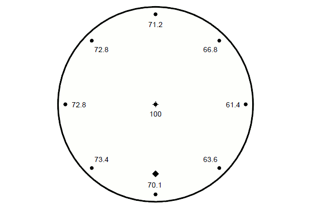
按照公式 \eqref{eq:10301a} 的要求,振幅必须取自变幅杆上"几何等效"位置的平均值 —— 即若观察者蒙住眼睛时转动变幅杆,这些位置彼此将无法区分。对于所有无型面圆柱形变幅杆,端面最小振幅出现在周边。对于圆柱体而言,周边任意位置都与其他周边位置无法区分。因此,选取八个等间距的周边位置(合理的采样),从菱形参考标记开始按顺时针方向,最小振幅的平均值为:
\begin{align} \label{eq:10306a} \overline{U}_{min} &= \frac{70.1 + 73.4 + 72.8 + 72.8 + 71.2 + 66.8 + 61.4 + 63.6} {8} \\ &=69.0 \nonumber \end{align}
因此,用于公式 \eqref{eq:10301a} 的平均最小振幅(69.0)大于最低的最小振幅(61.4)。
那么最大振幅呢?根据现有数据,最高振幅位于端面中心(100)。由于变幅杆上不存在与中心几何等效的其他位置,因此 100 微米就是最大振幅应采用的正确值。
于是,端面振幅均匀性为 —
\begin{align} \label{eq:10307a} \widehat{U} &= \frac{69.0}{100} \\[0.3em]%eqn_interline_spacing &=0.69 \nonumber \end{align}
如果在公式 \eqref{eq:10301a} 中使用的是最低最小振幅(61.4 微米)而不是平均最小振幅,则计算出的(错误的)均匀性将是:
\begin{align} \label{eq:10308a} \widehat{U} &= \frac{61.4}{100} \\[0.3em]%eqn_interline_spacing &=0.61 \nonumber \end{align}
测量次数
在上面的示例中,沿周边共进行了八次测量。若只进行四次测量,结果几乎相同。从最靠近菱形参考标记的位置开始,每隔一个读数取一次振幅(共四个),平均最小振幅为 68.9,对应的均匀性为 0.689。从参考标记顺时针方向的下一个测量点开始,每隔一个读数取一次振幅(共四个),平均最小振幅为 69.2,对应的均匀性为 0.692。因此,对于该变幅杆,四次振幅测量已经足够。
中心均匀性
在某些情况下,定义中心均匀性会比较方便。此时,参考振幅(公式 \eqref{eq:10301a} 分母中的振幅)取所选端面中心处的振幅,无论它是否为最大平均振幅:
\begin{align} \label{eq:10302a} \widehat{U}_{central} = \frac{\overline{U}_{min} \textsf{ or } \overline{U}_{max}}{\overline{U}_{central}} \end{align}
注意,分子并不一定使用螺柱中心线处的振幅。
该定义通常仅在表面上所有振幅都大于或都小于中心线振幅时使用。如果所有振幅都大于中心线振幅,则均匀性大于 1.0,称该表面存在振幅隆起。反之,如果所有振幅都小于中心线振幅,则均匀性小于 1.0,称该表面存在振幅下垂。
该定义对于绘制均匀性随另一参数(例如某个变更的变幅杆尺寸)变化的曲线特别有用。此类曲线的示例见 zzz。
接触均匀性
某些应用仅在端面的某些区域进行焊接(即变幅杆与塑料件接触的区域)。此时,整个端面的均匀性并不重要,只有接触区域内的均匀性才有意义。
周边均匀性
对于仅沿端面周边接触的变幅杆,周边均匀性为 —
\begin{align} \label{eq:10303a} \widehat{U}_{periphery} = \frac{\overline{U}_{min~(periphery)}}{\overline{U}_{max~(periphery)}} \end{align}
zzz 示例。该定义对于大型圆柱形和矩形变幅杆特别有用。
圆形区域均匀性
焊接圆形工件时,"显而易见"的选择是圆柱形变幅杆。然而,有时块形变幅杆的性能更好(例如接触区域内均匀性更好、频率分离度更好、寿命更长等)。在这种情况下使用块形变幅杆时,圆形接触区域内的均匀性为 —
\begin{align} \label{eq:10304a} \widehat{U}_{circular} = \frac{\overline{U}_{min~(within~circle)}}{\overline{U}_{max~(within~circle)}} \end{align}
特殊情况
考虑一种特殊情况:变幅杆存在相当严重的不对称性。图 zzz 给出了一个直径 100 mm 线轴形变幅杆端面上的振幅分布。最高端面振幅为 21.7 微米,实际上出现在端面边缘。我们是否应将此值作为公式 \eqref{eq:10301a} 中的最大振幅来计算均匀性?不应如此!请记住,必须对几何等效位置处的所有振幅取平均值。在本例中,另有七个振幅测量点,其位置(端面边缘处)与 21.7 微米测量点的位置几何等效。将这八个测量值平均后,结果为 17.7 微米。由于该值低于中心线振幅 19.3 微米,因此公式 \eqref{eq:10301a} 的分子应采用 17.3 微米,而分母应采用 19.3 微米。
如上述示例所示,在公式 ó1Â 中必须使用正确的数值来计算均匀性。如果不存在不对称性问题,那么只需在端面上找出单个最高振幅和单个最低振幅,即可直接算出均匀性。然而,由于大多数变幅杆都存在一定程度的不对称性,因此必须在几何等效位置进行多次振幅测量,然后取平均,以确定平均最小值和平均最大值。需要多少次测量?这取决于端面的几何形状。我们将在接下来的几节中举例说明。
采用平均振幅的理由
公式 \eqref{eq:10301a} 使用来自"几何等效位置"的平均振幅,而不是直接使用最小和最大振幅,原因有两个:
- 使用平均振幅可以揭示某些否则会被变幅杆不对称性所掩盖的均匀性关系。特别地,由公式 \eqref{eq:10301a} 给出的均匀性似乎合理地不受变幅杆不对称程度的影响。(支持这一结论的数据,请参见"实心、无槽圆柱形变幅杆的端面均匀性;不对称性对均匀性的影响"一节。)如果我们只是简单地将最小实测振幅除以最大实测振幅,情况就不是这样。
- 当变幅杆按名义相同尺寸加工时,它们的不对称性可能略有差异。使用平均振幅可以抹平这些不对称性,从而能够合理地将这些变幅杆的性能相互比较,或与设计略有不同的变幅杆进行比较。
不对称性
振幅不对称性(通常简称"不对称性")是衡量变幅杆上几何等效位置处振幅变化程度的指标。因此,对于振幅不对称的变幅杆,公式 \eqref{eq:10301a} 的均匀性计算只能部分描述其振幅性能,故还需要第二个参数(不对称性)。
不对称性定义为:
\begin{align} \label{eq:10305a} \textsf{Asymmetry} \widehat{A} = \frac{\textsf{Highest amplitude - Lowest amplitude}}{\textsf{Highest amplitude}} \end{align}
在该公式中,最大振幅和最小振幅都必须在同一表面上的几何等效位置处测得。此外,这些振幅是实际测量的振幅,而不是平均振幅。
与均匀性一样,不对称性既可以用小数表示,也可以用百分数表示。例如,不对称性 0.27 等价于 27%。本文一般采用小数形式。
再来看上面的 Ø100 mm 变幅杆,其端面周边的振幅并不均匀。最大振幅为 73.4,最小振幅为 61.4,不对称性为 —
\begin{align} \label{eq:10309a} \widehat{A} &= \frac{73.4 - 61.4}{73.4} \\[0.3em]%eqn_interline_spacing &=0.16 \nonumber \end{align}
对于设计良好的变幅杆,当几何等效位置处的所有振幅完全相等时,不对称性最佳,为 0.0。当最小振幅为 0 时,不对称性最差,为 1.0。
局限性
公式 \eqref{eq:10305a} 并不完全令人满意,因为它没有考虑不对称性所跨越的距离。例如,考虑一个在螺柱表面上不对称性为 0.2 的变幅杆。如果螺柱表面直径为 100 mm,则变幅杆接头仍可能有可接受的表现(取决于接头振幅)。然而,如果螺柱表面直径为 40 mm,则振幅梯度比 Ø100 mm 变幅杆要严重得多,因此该变幅杆接头的可靠性应当较低。不过,为避免不必要的复杂性,公式 \eqref{eq:10305a} 似乎是合理的。无论如何,不对称性总是可以针对某个特定的关注区域(例如接头)来规定(如 \( \widehat{A}_{joint} \))。
(注意:计算均匀性或不对称性时,只使用振幅的大小,不要使用与振幅相位相关的正负号。振幅相位将在"振型分析"一章中介绍。)
均匀性计算(高级)
尽管公式 \eqref{eq:10301a} 实现起来相当容易且结果一致,但它与变幅杆性能的相关性可能并不特别好。这是因为性能取决于指定表面上的振幅分布,而不仅仅是最大和最小振幅。参见附录 A。
一个与变幅杆性能相关性更好的均匀性定义为 —
其中新定义的均匀性为 —
\begin{align} \label{eq:10320a} \widehat{U}' = \frac{\overline{U}} {\overline{U}_{max}} \end{align}
式中 —
| \( \widehat{U}' \) | = 均匀性(高级) |
| \( \overline{U} \) | = 指定表面上所有轴向振幅的平均值 |
| \( \overline{U}_{max} \) | = 指定表面上最大轴向振幅的平均值(同前) |
附录 A
公式 \eqref{eq:10301a} 的局限性
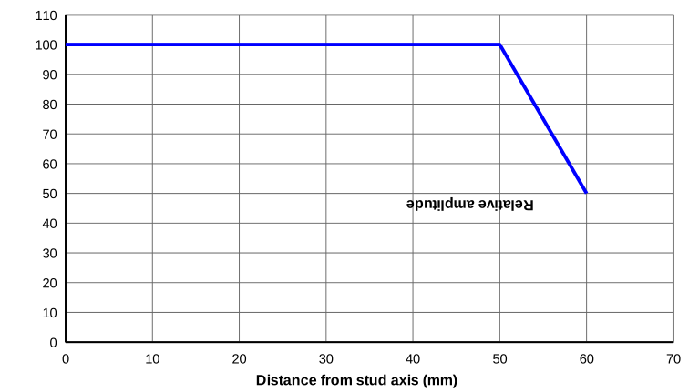
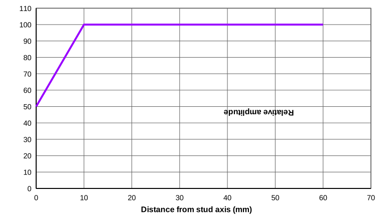
下面的各图展示了三种 120 mm 平端面变幅杆设计的假想振幅分布。这种不连续的振幅分布在实际变幅杆中不会出现,但可用来说明公式 \( \usetagform{} \eqref{eq:10301a} \usetagform{A} \) 的局限性,为方便起见,该公式重列如下。
\begin{align} \label{eq:10349a} \widehat{U} = \frac{\overline{U}_{min}}{\overline{U}_{max}} \end{align}
注意,振幅分布从螺柱轴线(即端面中心)开始,因此振幅分布的范围是从 0(螺柱轴线)到 60 mm。
|
|
|
|
|
|
|
|
|
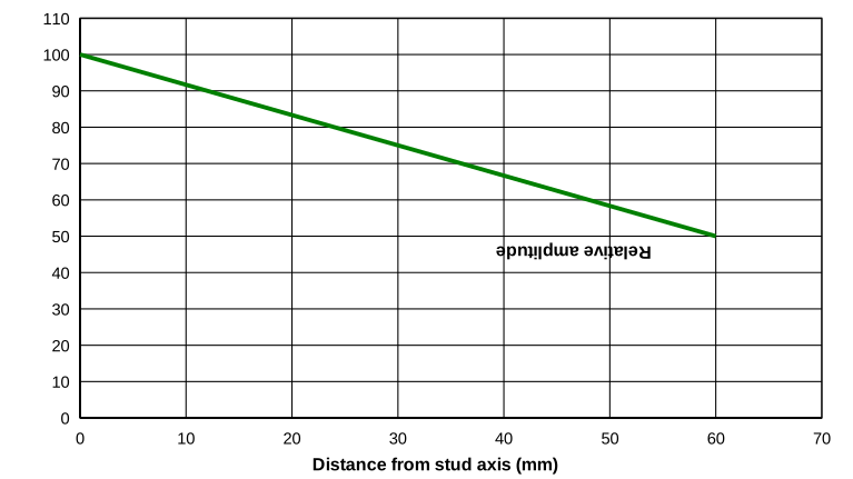
使用公式 \eqref{eq:10349a} 时,所有这些变幅杆具有相同的 \( \overline{U}_{min} \) (50)和相同的 \( \overline{U}_{max} \) (100),因此均匀性相同(0.50)。然而,显而易见的是,变幅杆 C 的性能将劣于另外两个变幅杆。变幅杆 A 与变幅杆 B 的性能彼此也可能不同,但这尚待验证。注意:即使将变幅杆设计 C 改造成设计 A(例如通过机加工),计算出的均匀性也不会改变,尽管其性能显然会有所改善。
下面说明如何从输送功率能力的角度对每个变幅杆的应用性能进行数值评估。首先,将端面在概念上划分为大量(n 个)小面积 \( A_i \)。则从每个小面积提取的局部功率 \( P_i \) 为 —
\begin{align} \label{eq:10351a} P_i = I_i \, A_i \end{align}
式中 —
| \( P_i \) | = 局部功率 |
| \( k \) | = 比例常数 |
| \( A_i \) | = 局部面积 |
局部功率强度由下式给出 —
\begin{align} \label{eq:10351a1} I_i = \frac{P_i}{A_i} \end{align}
变幅杆整个表面上的总功率 \( P \) 就是全部 n 个局部功率之和(∑):
\begin{align} \label{eq:10352a} P = \sum{I_i \, A_i} \end{align}
一个均匀性较差的大型变幅杆仍可能比均匀性良好的小型变幅杆输送更大的功率。因此,为了正确比较两个面积不同的变幅杆的性能,必须将功率除以变幅杆与流体之间的接触(端面)面积。由此得到端面上的平均功率 —— 即功率强度 \( \overline{I} \):
\begin{align} \label{eq:10353a} \overline{I} &= \frac{P}{A} \\[0.7em]%eqn_interline_spacing &= \left[\frac{\sum{I_i \, A_i}}{A}\right] \nonumber \end{align}
式中 —
| \( \overline{I} \) | = 平均功率强度 |
| \( P \) | = 从端面接触面积辐射的总功率 |
| \( A \) | = 端面总接触面积 |
公式 \eqref{eq:10353a} 完全具有一般性。现在为简便起见,假设变幅杆在发生空化的流体中工作。对于空化负载,功率或强度与振幅成正比。(参见 Peshkovsky,图 9,第 321 页。)此时公式 \eqref{eq:10353a} 可写为 —
\begin{align} \label{eq:10353a1} \overline{I} &= \left[\frac{\sum{(k_i \, U_i) \, A_i}}{A}\right] \end{align}
式中 —
| \( U_i \) | = 局部面积 \( A_i \) 处的振幅 |
| \( k_i \) | = 振幅 \( A_i \) 与强度 \( I_i \) 之间的比例常数 |
比例常数 \( k_i \) 取决于流体种类、温度和压力等因素。对于空化而言,这些因素可认为在整个空化表面上为常数。然而,由于边缘效应(即在相同振幅下,边缘处产生的空化可能较少),\( k_i \) 在靠近边缘处可能并非常数。在本次均匀性分析中将忽略这种可能的边缘效应。于是 \( k_i \) 可认为在空化表面上处处相等,并可移到求和号之外。
\begin{align} \label{eq:10353a2} \overline{I} &= k \, \left[\frac{\sum{U_i \, A_i}}{A}\right] \end{align}
量 \( \left[\frac{\sum{U_i \, A_i}}{A}\right] \) 正是负载表面(通常为端面)上振幅 \( U_i \) 的平均值。
\begin{align} \label{eq:10354a} \overline{U} = \left[\frac{\sum{U_i \, A_i}}{A}\right]\end{align}
式中 —
| \( \overline{U} \) | = 指定表面上的平均轴向振幅 |
于是公式 \eqref{eq:10353a1} 可写为 —
\begin{align} \label{eq:10355a} \overline{I} = k \, \overline{U} \end{align}
因此,空化负载的强度与平均端面振幅 \( \overline{U} \) 成正比。
为了比较两个工作在不同振幅下的变幅杆,应将 \( \overline{I} \) 除以变幅杆的平均最大振幅 \( \overline{U}_{max} \)。于是,将公式 \eqref{eq:10355a} 两边同除以 \( \overline{U}_{max} \) 得:
\begin{align} \label{eq:10356a} \overline{I}' &= \frac{\overline{I}}{\overline{U}_{max}} \\[0.7em]%eqn_interline_spacing &= k \, \frac{\overline{U}} {\overline{U}_{max}} \nonumber \\[0.7em]%eqn_interline_spacing &= k \, \widehat{U}' \nonumber \end{align}
式中 —
| \( \overline{I}' \) | = 单位振幅的平均强度 |
| \( \overline{U}_{max} \) | = 指定表面上最大轴向振幅的平均值 |
其中新定义的均匀性为 —
\begin{align} \label{eq:10357a} \boxed{ \widehat{U}' = \frac{\overline{U}} {\overline{U}_{max}} } \end{align}
此均匀性记为 \( \widehat{U}' \),以区别于公式 \eqref{eq:10349a} 中原来的 \( \widehat{U} \)。该定义与公式 \eqref{eq:10349a} 非常相似,只是分子 \( \overline{U} \) 是整个端面上的平均振幅,而不是端面振幅最小值的平均 \( {U}_{min} \)。然而现在,该定义满足了变幅杆性能应与均匀性相关的要求 —— 即对于两个归一化最大端面振幅相同的变幅杆,均匀性 \( \widehat{U}' \) 较大者将具有更高的平均功率强度 \( \overline{I}' \)。
与公式 \eqref{eq:10349a} 的比较
对于上文图 A1 至图 A3 中的假想变幅杆,所假设的变幅杆形状既可以是矩形的,也可以是圆柱形的。由公式 \eqref{eq:10349a} 和 \eqref{eq:10357a} 计算出的均匀性列于表 A1,并在下文讨论。
当使用公式 \eqref{eq:10349a} 评估均匀性时,无论振幅分布或变幅杆形状如何,所有变幅杆的均匀性都相同。因此,公式 \eqref{eq:10349a} 无法指出哪个变幅杆性能最好。相比之下,公式 \eqref{eq:10357a} 的均匀性有助于按照性能区分这些变幅杆。
矩形变幅杆
对于矩形变幅杆,公式 \eqref{eq:10354a} 中的局部面积 \( A_i \) 就是 \( t \, Δx \),其中 \( t \) 为端面厚度,\( Δx \) 为沿变幅杆宽度方向的小增量。(为简便起见,此处假设变幅杆振幅沿端面厚度方向恒定。)于是变幅杆 A 和 B 的均匀性相等(0.958),将输送相等的空化功率,而变幅杆 C 的均匀性较低(0.750),输送的空化功率较低。
圆柱形变幅杆
对于圆柱形变幅杆,公式 \eqref{eq:10354a} 中的局部环形面积 \( A_i \) 为 \( 2π r Δr \),其中 \( r \) 为计算 \( A_i \) 处的半径,\( Δr \) 为以 \( r \) 为中心的小增量。尽管所有圆柱形变幅杆的物理端面面积相同,但所输送的功率不仅取决于局部振幅,还取决于输送功率处的局部环形面积。变幅杆 B 在其周边处具有 100 的相对振幅,而该处变幅杆的环形面积最大。相比之下,变幅杆 A 在这一关键区域的相对振幅较低。(变幅杆 A 在螺柱轴线附近确实具有更好的相对振幅,但由于该区域的环形面积较小,故效果较差。)
因此,变幅杆 B 的均匀性最高(0.995),其次是变幅杆 A(0.921)。变幅杆 C 再次垫底,但其由公式 \eqref{eq:10357a} 算出的均匀性(0.667)仍优于由公式 \eqref{eq:10349a} 算出的结果(0.5)。
为了对圆柱形变幅杆获得更直观的感受,可以考虑若干圆柱形桶,每个桶中都装满沙子至最大高度 h。每个桶顶部沙子的分布方式与振幅分布相同。沙子最多的桶(最重的桶)将最接近"理想"桶——即沙子顶部完全平坦的桶。桶 B 的沙子最多,其次是桶 A,然后是桶 C。事实上,桶 B 的沙子量将达到沙子完全平坦的桶的 99.5%。
特殊情形 — 所有 \( A_i \) 相等
公式 \eqref{eq:10354a} 存在一个特殊情形:所有小的局部面积 \( A_i \) 都相等;称该小面积为 \( A_0 \)。由于 \( A_0 \) 是固定的,无需与某个特定的 \( U_i \) 相关联,因此可以移到求和号之外。于是公式 \eqref{eq:10354a} 变为:
\begin{align} \label{eq:10358a} \overline{U} &= \frac{A_0\sum{U_i}}{A} \\[0.7em]%eqn_interline_spacing &= \frac{\sum{U_i}}{(A/A_0)} \nonumber \end{align}
\( A/A_0 \) 就是需要计算振幅的位置总数 \( n \)。于是公式 \eqref{eq:10358a} 变为:
\begin{align} \label{eq:10359a} \overline{U} &= \left( \sum{U_i} \right)/n \end{align}
公式 \eqref{eq:10359a} 相对于公式 \eqref{eq:10354a} 的优势在于无需考虑各个局部面积 \( A_i \)。事实上,公式 \eqref{eq:10359a} 与变幅杆接触面积完全无关。因此,对于测量点等间距的扫描激光测振仪,或网格相对均匀的有限元分析,将公式 \eqref{eq:10359a} 代入公式 \eqref{eq:10357a} 即可相当容易地计算出均匀性:
\begin{align} \label{eq:10360a} \widehat{U}' &= \frac{\left( \sum{U_i} \right)/n} {\overline{U}_{max}} \end{align}
实现中的问题
尽管公式 \eqref{eq:10357a} 和 \eqref{eq:10360a} 在概念上很有吸引力,但在实践中可能难以实现。
实验方法
对于实验测量而言,主要问题之一是为确定平均端面振幅 \( \overline{U} \) 所需获取的振幅 \( U_i \) 数据量很大,尤其是当变幅杆存在振幅不对称性时。例如,对于一个 20 kHz 变幅杆,假设必须以 10 mm 的网格间距确定振幅。(这个间距实际上可能偏大,但可供讨论之用。)下表给出了各种变幅杆所需的振幅测量次数。
|
|||||||||||||||
|
表中的第一个变幅杆是条形变幅杆。由于 15 mm 的端面厚度相对较小,振幅沿厚度方向不应有太大变化。此时只需沿变幅杆宽度方向以 10 mm 间隔进行振幅测量,这完全可以手动移动振幅探头来完成。
其余变幅杆的横向尺寸都很大,因此需要在整个端面上测定振幅。这对于手动定位的探头来说并不现实,此时需要某种全场测量方法。
(上表假设需要在整个端面上进行振幅测量,这可能是因为存在振幅不对称性。如果假设不对称性可以忽略,则只需在端面的一个局部区域测量振幅。例如,仅测量四分之一区域可能就足够了。)
直接振幅测量
公式 \eqref{eq:10357a} 是基于将变幅杆均匀性与水中空化负载相关联的能力推导出来的。因此,可以按以下步骤比较两种变幅杆设计的相对均匀性。
- 在空气中测量超声叠堆的功率。
- 将端面浸入合适容器中经脱气的室温水中。
- (根据需要)增大振幅,直至端面上出现充分空化。
- 测量功率。
- 在空气中、电源设置不变的情况下,测量变幅杆的最高平均振幅。
- 由公式 \eqref{eq:10357a} 或 \eqref{eq:10360a} 计算强度。
该步骤存在若干困难。
- 该步骤不能给出均匀性的绝对度量,而是给出一个与均匀性相关的强度值。因此,它仅适用于比较不同变幅杆的相对性能。
- 水中测得的功率不仅来自变幅杆的轴向振幅,还来自变幅杆浸入部分的周边处的横向振幅。因此,仅取决于端面振幅轴向均匀性的那部分功率无法独立确定(除非横向振幅很小,此时由横向振幅引起的空化功率可以忽略)。
- 公式 \eqref{eq:10353a2} 及后续公式是在忽略边缘效应的假设下推导的。此类效应很可能存在,但其相对影响未知(除了在边缘面积与端面面积之比更大的小型变幅杆中可能更显著之外)。
- 由于必须浸入整个端面,该步骤不适用于测量端面局部区域的均匀性。
- 电源必须有足够的功率来引发空化,这在评估较大变幅杆时可能是个问题。
- 必须注意确保变幅杆的其他结构(如槽、沟槽等)不被浸没,因为这些结构会产生无法计入的额外空化功率。
- 该方法的可重复性值得怀疑,尤其是当在不同实验室使用不同设备进行测量时。
解析方法(计算机仿真)
对于有限元计算机仿真,振幅值可以很容易地从有限元网格节点获取。然而,困难依然存在。
- 公式 \eqref{eq:10360a} 仅在振幅测量位置彼此等间距、从而所有局部 \( A_i \) 相同时才适用。在有限元分析中,很多情况下并非如此。例如,当槽离端面较近时,槽端附近的端面网格会比周围网格更细。此时不能使用公式 \eqref{eq:10360a},因为较细的局部网格会产生不当的影响;而必须使用公式 \eqref{eq:10357a}。然而,公式 \eqref{eq:10357a} 涉及平均振幅 \( \overline{U} \)(公式 \eqref{eq:10354a}),只有能为每个局部振幅 \( U_i \) 确定相应的局部面积 \( A_i \) 时才能计算。然而,\( A_i \) 通常无法直接从有限元结果中获得,因为节点本身没有面积;只有单元面才有面积。不过,所需的 \( A_i \) 也许可以通过对有限元原始数据进行处理来获得(例如,由与节点 i 相邻的单元面计算 \( A_i \))。
- 当有限元只分析变幅杆的一个局部区域(例如圆柱形变幅杆的四分之一区域)时,公式 \eqref{eq:10357a} 会对局部区域边界上节点的振幅赋予全权重。实际上,这些振幅只应赋予半权重,因为在完整模型中,这些节点实际上由相邻区域共享。因此,对局部区域用公式 \eqref{eq:10357a} 计算的均匀性,与将公式 \eqref{eq:10357a} 应用于整个端面所得的均匀性并不一致。不过,只要边界节点数相对于端面节点总数较少,偏差就会很小。(对于端面周边处的节点也可以作类似论证,因为此类节点对应的面积仅为内部节点的一半。)
- 对于轴对称有限元模型,无法获得整个端面,只能获得沿端面一条径线上的振幅。为了计算均匀性,必须按下式计算每个节点对应的环形面积:
\begin{align} \label{eq:10361a} A_i =2\pi \, r_i \, w_i \end{align}
式中 —
\( A_i \) = 节点 i 处单元的环形面积 \( r_i \) = 节点 i 到端面中心线的径向距离 \( w_i \) = 节点 i 处单元的径向宽度 每个 \( w_i \) 可以基于相邻节点的半径(\( r_{i+1} \) 和 \( r_{i-1} \))取平均值来计算:
\begin{align} \label{eq:10362a} w_i &= \frac{r_{i+1} + r_i} {2} - \frac{r_{i} + r_{i-1}} {2} \\[0.7em]%eqn_interline_spacing &= \frac{r_{i+1} - r_{i-1}} {2} \nonumber \end{align}
式中 —
\( r_{i+1} \), \( r_{i-1} \) = 与节点 i 相邻的节点的半径 对于中心线节点和端面周边节点,必须特别处理。
公式 \eqref{eq:10361a} 最好通过将轴对称振幅及相应半径导出到外部软件(如电子表格)中来进行计算。
因此,尽管公式 \eqref{eq:10357a} 在概念上优于公式 \eqref{eq:10349a},但由于上述问题,它可能并不实用。
Amplitude uniformity and asymmetry — calculations
Contents
- Uniformity calculation (basic)
- Asymmetry
- Appendix A - Limitations of Equation 1
- Also see — Uniformity — basic concepts
- Figures
This section will look at how amplitude uniformity and asymmetry are calculated. (For an introduction see Uniformity — Basic Concepts.)
Uniformity calculation (basic)
A calculated value of uniformity should have the following characteristics:
- It should be relatively easy to determine (implement).
- It should correlate strongly to the performance of the horn (i.e., a horn with a high uniformity should perform better than an equivalent horn with low uniformity).
- It should allow easy comparison among various data sources (empirical amplitude measurements, FEA 3D, FEA axisymmetric, etc.).
- It should be repeatable.
The simplest equation for uniformity is —
\begin{align} \label{eq:10301a} \widehat{U} = \frac{\overline{U}_{min}}{\overline{U}_{max}} \end{align}
where —
| \( \widehat{U} \) | = uniformity |
| \( \overline{U}_{min} \) | = average of minimum axial amplitudes on a specified surface |
| \( \overline{U}_{max} \) | = average of maximum axial amplitudes on a specified surface |
Notes:
- Depending on the circumstances, uniformity can be expressed either as a decimal value or as a percent. For example, a uniformity of 0.92 is equivalent to a uniformity of 92%. Here the decimal value will generally be used.
- Unless otherwise specified, all amplitudes used to calculate the uniformity are axial.
- The "specified surface" will typically be the output surface. Occasionally (as will be indicated) the "specified surface" will be the input surface (e.g., when dealing with joint problems).
- The "specified surface" may not necessarily encompass the entire surface. See Contact uniformity below.
- \( \overline{U}_{min} \) is the average from symmetric (geometrically equivalent) locations on the specified surface where the amplitudes are a minimum; similarly for \( \overline{U}_{max} \). This is necessary because horns sometimes have asymmetric amplitude distributions, even though the horn itself is nominally symmetric with respect to the stud axis. This will become clearer below with some examples.
- The uniformity calculated from equation \eqref{eq:10301a} will always have a value less than or equal to 1.0. (Note: the central uniformity (below) may have a value greater than 1.0.)
- Well-designed horns should have high uniformity. Therefore, the best possible uniformity will be 1.0 (i.e., where every face amplitude is identical). The worst possible uniformity will be 0.0 when the minimum amplitude is zero. If the specified surface has a node then the uniformity is automatically zero.
Example 1: Ø101 mm unshaped, unslotted, solid cylindrical horn
For a particular 20 kHz Ø101 mm unshaped solid cylindrical horn, the measured relative amplitudes are shown in figure 1.
|
|
|
According to the requirements of equation \eqref{eq:10301a}, the amplitudes must be averaged from locations on the horn that are "geometrically equivalent" — i.e., locations that would not be distinguishable from each other if the horn were rotated while an observer were blindfolded. For all unshaped cylindrical horns, the minimum face amplitude will be at the periphery. For a cylinder, any peripheral location is indistinguishable from any other peripheral location. Therefore, choosing eight equally spaced peripheral locations (a reasonable sample), the average minimum amplitude is (proceeding clockwise from the diamond reference mark):
\begin{align} \label{eq:10306a} \overline{U}_{min} &= \frac{70.1 + 73.4 + 72.8 + 72.8 + 71.2 + 66.8 + 61.4 + 63.6} {8} \\ &=69.0 \nonumber \end{align}
Thus, the average minimum amplitude (69.0) to be used in equation \eqref{eq:10301a} is greater than the least minimum amplitude (61.4).
What about the maximum amplitude? From the available data, the highest amplitude is at the center of the horn face (100). Since there is no other location on the horn that is geometrically equivalent to the center, then 100 microns is the correct value to use for the maximum amplitude.
Thus, the face amplitude uniformity is —
\begin{align} \label{eq:10307a} \widehat{U} &= \frac{69.0}{100} \\[0.3em]%eqn_interline_spacing &=0.69 \nonumber \end{align}
If the least minimum amplitude (61.4 microns) had been used in equation \eqref{eq:10301a} (rather than the averaged minimum) then the calculated (incorrect) uniformity would have been:
\begin{align} \label{eq:10308a} \widehat{U} &= \frac{61.4}{100} \\[0.3em]%eqn_interline_spacing &=0.61 \nonumber \end{align}
Number of measurements
In the above example, eight measurements were made around the periphery. Using only four measurements would have given nearly the same results. Starting at the location closest to the diamond reference mark and taking every other amplitude reading (four total), the averge minimum amplitude is 68.9 for which the uniformity is 0.689. Starting at the measurement just clockwise from the reference mark and taking every other amplitude reading (four total), the averge minimum amplitude is 69.2 for which the uniformity is 0.692. Hence, four amplitude measurements would have been sufficient for this horn.
Central uniformity
In some cases it is convenient to define a the central uniformity. In this case, the reference amplitude (in the denominator of equation \eqref{eq:10301a}) is the amplitude at the center of the chosen face, regardless if this is the largest average amplitude:
\begin{align} \label{eq:10302a} \widehat{U}_{central} = \frac{\overline{U}_{min} \textsf{ or } \overline{U}_{max}}{\overline{U}_{central}} \end{align}
Note that the stud centerline amplitude is not necessarily used for the numerator.
This definition is normally used only when all of the surface amplitudes are either larger or smaller than the centerline amplitude. If all of the amplitudes are larger than the centerline amplitude, then the uniformity will be greater than 1.0 and the surface is said to have amplitude rise. Conversely, if all of the amplitudes are smaller than the centerline amplitude, then the uniformity will be less than 1.0 and the surface is said to have amplitude droop.
This definition is especially useful for plotting graphs of uniformity versus another parameter (e.g., an altered horn dimension). See zzz for an example of this type of graph.
Contact uniformity
Some applications are welded only along in certain areas of the horn face (i.e., where the horn contacts the plastic part). Then the overall face uniformity is not important; only the uniformity over the contact area matters.
Peripheral uniformity
For a horn that contacts only around the periphery of the face, the peripheral uniformity is —
\begin{align} \label{eq:10303a} \widehat{U}_{periphery} = \frac{\overline{U}_{min~(periphery)}}{\overline{U}_{max~(periphery)}} \end{align}
zzz Example. This definition is especially useful for large cylindrical and rectangular horns.
Circular uniformity
When welding a circular part the "obvious" choice is a cylindrical horn. However, sometimes a block horn will have better performance (e.g., better uniformity over the contact area, better frequency separation, better life, etc.). When a block horn is thus used, the uniformity within the circular contact area is —
\begin{align} \label{eq:10304a} \widehat{U}_{circular} = \frac{\overline{U}_{min~(within~circle)}}{\overline{U}_{max~(within~circle)}} \end{align}
Peculiarities
Consider a peculiar situation in which the horn has rather extreme asymmetry. Figure zzz shows the amplitude distribution on the face of a 100 mm diameter spool horn. The highest face amplitude is 21.7 microns, which actually occurs at the edge of the horn face. Should we use this value as the maximum amplitude in equation \eqref{eq:10301a} to calculate the uniformity? No! Remember that you must find an average of all amplitudes at locations that are geometrically equivalent. In this case, there are seven other amplitude measurements whose locations (at the edge of the horn face) are geometrically equivalent to that of the 21.7 micron measurement. When all eight of these measurements are averaged, the result is 17.7 microns. Since this value is lower than the centerline amplitude of 19.3 microns, then 17.3 microns is the value to use in the numerator of equation \eqref{eq:10301a}, while 19.3 microns should be used in the denominator.
As the above examples show, you must be careful to use the correct values in equation ó1Â to calculate the uniformity. If asymmetry were not a problem, then you could just search the horn face for a single highest and lowest amplitude, from which the uniformity could be directly calculated. However, since most horns have some asymmetry you must take multiple amplitude measurements at geometrically equivalent locations, which are then averaged to determine the average minimum and maximum values. How many measurements are needed? This will depend on the geometry of the horn face. We will look at examples in the next sections.
Justification for averaged amplitudes
Equation \eqref{eq:10301a} uses averaged amplitudes from "geometrically equivalent locations" rather than just using the smallest and largest amplitudes. There are two reasons:
- Using averaged amplitudes exposes certain uniformity relations that would otherwise be obscured by the horn asymmetry. In particular, it appears that the uniformity as given in equation \eqref{eq:10301a} is reasonably unaffected by the amount of horn asymmetry. (For data that supports this conclusion, see the section on "Face Uniformity for Solid, Unslotted Cylindrical Horns; Effect of Asymmetry on Uniformity".) This is not true if we simply divide the smallest measured amplitude by the largest measured amplitude.
- When horns are machined to nominally identical dimensions, they may have somewhat different asymmetries. Using averaged amplitudes smoothes out these asymmetries so that the performance of these horns can reasonably be compared to each other or to horns of somewhat different designs.
Asymmetry
Amplitude asymmetry (generally just "asymmetry") is a measure of how much the amplitude varies at geometrically equivalent locations on the horn. Then for a horn with asymmetric amplitude, the uniformity calculation of equation \eqref{eq:10301a} only partially describes the amplitude performance. Therefore, a second parameter (asymmetry) is needed.
Asymmetry is defined as:
\begin{align} \label{eq:10305a} \textsf{Asymmetry} \widehat{A} = \frac{\textsf{Highest amplitude - Lowest amplitude}}{\textsf{Highest amplitude}} \end{align}
In this equation, both the maximum and minimum amplitude must be measured on the same surface from geometrically equivalent locations. Also, these amplitudes are the actual measured amplitudes, not averaged amplitudes.
As with uniformity, asymmetry can be expressed either as a decimal value or as a percent. For example, an asymmetry of 0.27 is equivalent to an asymmetry of 27%. Here the decimal value will generally be used.
Looking again at the above Ø100 mm horn, the amplitude is not uniform at the periphery of the horn face. With a maximum amplitude of 73.4 and a minimum amplitude of 61.4, the asymmetry is —
\begin{align} \label{eq:10309a} \widehat{A} &= \frac{73.4 - 61.4}{73.4} \\[0.3em]%eqn_interline_spacing &=0.16 \nonumber \end{align}
For well-designed horns, the best possible asymmetry will be 0.0 when all amplitudes from geometrically equivalent locations are exactly equal. The worst possible asymmetry will be 1.0 when the minimum amplitude is 0.
Limitations
Equation \eqref{eq:10305a} is not entirely adequate because it doens't consider the distance over which the asymmetry occurs. For example, consider a horn that has an asymmetry of 0.2 over the stud surface. If the diameter of the stud surface is 100 mm then the horn joint might still perform acceptably (depending on the joint amplitude). However, if the diameter of the stud surface is 40 mm then the amplitude gradient is much more severe that for the Ø100 mm horn so the horn joint should be less reliable. However, equation \eqref{eq:10305a} seems reasonable in order to avoid undue complexity. In any case, the asymmetry can simply be specified for a particular region of interest such as the joint (e.g., as \( \widehat{A}_{joint} \)).
(Note: when calculating either the uniformity or the asymmetry, use only the magnitude of the amplitudes. Do not use the sign that is associated with the phase of the amplitude. The amplitude phase is covered in the chapter on "Modeshape Analysis".)
Uniformity calculation (advanced)
Although equation \eqref{eq:10301a} is fairly easy to implement and gives consistent results, the correlation with horn performance may not be particularly good. This is because the performance depends on the amplitude distribution across the specified surface, not just the maximum and minimum amplitudes. See Appendix A.
A definition of uniformity that correlates more closely to the horn's performance is —
and where the newly defined uniformity is —
\begin{align} \label{eq:10320a} \widehat{U}' = \frac{\overline{U}} {\overline{U}_{max}} \end{align}
where —
| \( \widehat{U}' \) | = uniformity (advanced) |
| \( \overline{U} \) | = average of all axial amplitudes on a specified surface |
| \( \overline{U}_{max} \) | = average of maximum axial amplitudes on a specified surface (as before) |
Appendix A
Limitations of Equation \eqref{eq:10301a}
The following figures show hypothetical amplitude distributions for three 120 mm flat faced horn designs. Such discontinuous amplitude distributions would not be seen in actual horns but serve to show the limitations of equation \( \usetagform{} \eqref{eq:10301a} \usetagform{A} \), repeated here for convenience.
\begin{align} \label{eq:10349a} \widehat{U} = \frac{\overline{U}_{min}}{\overline{U}_{max}} \end{align}
Note that the amplitude distribution starts from the stud axis (i.e., the center of the horn's face) so the amplitude distribution goes from 0 (the stud axis) to 60 mm.
|
|
|
|
|
|
|
|
|
Using equation \eqref{eq:10349a} all of these horns have the same \( \overline{U}_{min} \) (50) and the same \( \overline{U}_{max} \) (100) and so all have the same uniformity (0.50). However, it seems rather obvious that horn C will perform worse than the other two horns. The performance of horn A and horn B may also be different from each other but this remains to be seen. Note: even if horn design C were transformed into design A (e.g., by machining), the calculated uniformity would not change even though the performance would have obviously have improved.
The following shows how the application performance of each horn can be evaluated numerically in terms of its ability to deliver power. First, consider that the horn face is conceptually divided into a large number n of small areas \( A_i \). Then the local power \( P_i \) that is drawn from each of these small areas is —
\begin{align} \label{eq:10351a} P_i = I_i \, A_i \end{align}
where —
| \( P_i \) | = local power |
| \( k \) | = proportionality constant |
| \( A_i \) | = local area |
and the local power intensity is given by —
\begin{align} \label{eq:10351a1} I_i = \frac{P_i}{A_i} \end{align}
The total power \( P \) over the entire surface of the horn is just the sum (∑) of all of the n local powers:
\begin{align} \label{eq:10352a} P = \sum{I_i \, A_i} \end{align}
It is possible that a large horn with poor uniformity may still deliver more power than a small horn having good uniformity. Therefore, to properly compare the performance of two horns having different areas, the power must be divided by the contact (face) area between the horn and the fluid. This gives the average power over the horn face — i.e., the power intensity \( \overline{I} \):
\begin{align} \label{eq:10353a} \overline{I} &= \frac{P}{A} \\[0.7em]%eqn_interline_spacing &= \left[\frac{\sum{I_i \, A_i}}{A}\right] \nonumber \end{align}
where —
| \( \overline{I} \) | = average power intensity |
| \( P \) | = total power radiated from the face contact area |
| \( A \) | = total face contact area |
Equation \eqref{eq:10353a} is perfectly general. Now for simplicity assume that the horn is operating in a cavitating fluid. For a cavitation load the power or intensity is directly proportional to the amplitude. (See Peshkovsky, figure 9, p. 321.) In this case equation \eqref{eq:10353a} can be written as —
\begin{align} \label{eq:10353a1} \overline{I} &= \left[\frac{\sum{(k_i \, U_i) \, A_i}}{A}\right] \end{align}
where —
| \( U_i \) | = amplitude at local area \( A_i \) |
| \( k_i \) | = proportionality constant between amplitude \( A_i \) and intensity \( I_i \) |
The proportionality constant \( k_i \) depends on factors such as the kind of fluid, the temperature and pressure, etc. For cavitation these factors can be considered to be constant across the cavitating surface. However, \( k_i \) may not be constant near the edge because of edge effects (i.e., for equal amplitudes an edge may produce less cavitation). Such possible edge effects will be ignored for this analysis of uniformity. Then \( k_i \) can be considered equal everywhere on the cavitating surface and can be moved outside the summation.
\begin{align} \label{eq:10353a2} \overline{I} &= k \, \left[\frac{\sum{U_i \, A_i}}{A}\right] \end{align}
The quantity \( \left[\frac{\sum{U_i \, A_i}}{A}\right] \) is just the average of the amplitudes \( U_i \) over the load surface (typically the face).
\begin{align} \label{eq:10354a} \overline{U} = \left[\frac{\sum{U_i \, A_i}}{A}\right]\end{align}
where —
| \( \overline{U} \) | = average axial amplitude over the specified surface |
Thus equation \eqref{eq:10353a1} can be written as —
\begin{align} \label{eq:10355a} \overline{I} = k \, \overline{U} \end{align}
Hence, the intensity from a cavitating load is directly proportional to the average face amplitude \( \overline{U} \).
In order to compare two horns operating at different amplitudes, \( \overline{I} \) should be divided by the horn's average maximum amplitude \( \overline{U}_{max} \). Thus, dividing both sides of equation \eqref{eq:10355a} by \( \overline{U}_{max} \) gives:
\begin{align} \label{eq:10356a} \overline{I}' &= \frac{\overline{I}}{\overline{U}_{max}} \\[0.7em]%eqn_interline_spacing &= k \, \frac{\overline{U}} {\overline{U}_{max}} \nonumber \\[0.7em]%eqn_interline_spacing &= k \, \widehat{U}' \nonumber \end{align}
where —
| \( \overline{I}' \) | = average intensity per unit amplitude |
| \( \overline{U}_{max} \) | = average of maximum axial amplitudes over the specified surface |
and where the newly defined uniformity is —
\begin{align} \label{eq:10357a} \boxed{ \widehat{U}' = \frac{\overline{U}} {\overline{U}_{max}} } \end{align}
This uniformity is designated as \( \widehat{U}' \) to distinguish it from the original \( \widehat{U} \) of equation \eqref{eq:10349a}. This definition is very similar to equation \eqref{eq:10349a} except that the numerator \( \overline{U} \) is the average amplitude over the entire horn face rather than the average of the face amplitude minimums \( {U}_{min} \). Now, however, this definition satisfies the requirement that the horn's performance should correlate to the uniformity — i.e., for two horns with the same normalized maximum face amplitudes, the one with the greatest uniformity \( \widehat{U}' \) will have the highest average power intensity \( \overline{I}' \).
Comparison to equation \eqref{eq:10349a}
For the above hypothetical horns of figures A1 through A3, the assumed horn shape could either be rectangular or cylindrical. The calculated uniformities from equations \eqref{eq:10349a} and \eqref{eq:10357a} are shown in table A1 and are discussed below.
|
||||||||||||||||||||||||||||
|
When equation \eqref{eq:10349a} is used to evaluate the uniformity, all of the horns have the same uniformity, regardless of the amplitude distribution or the horn shape. Therefore, equation \eqref{eq:10349a} gives no indication of which horn will perform best. In contrast, the uniformity from equation \eqref{eq:10357a} helps to distinguish the horns according to their performance.
Rectangular horns
For a rectangular horn the local area \( A_i \) in equation \eqref{eq:10354a} is just \( t \, Δx \) where \( t \) is the face thickness and \( Δx \) is a small increment along the horn's width. (For simplicity here, the horn's amplitude is assumed to be constant across the face thickness.) Then horns A and B have equal uniformities (0.958) and will deliver equal cavitation power, whereas horn C is less uniform (0.750) and will deliver lower cavitation power.
Cylindrical horns
For a cylindrical horn the local circular area \( A_i \) in equation \eqref{eq:10354a} is \( 2π r Δr \) where \( r \) is the radius where \( A_i \) is being evaluated and \( Δr \) is a small increment centered at \( r \). Even though all of the cylindrical horns have the same physical face area, the delivered power depends not only on the local amplitude but also on the local circular area where the power is delivered. Horn B has 100 relative amplitude at its periphery where the circular area of the horn is greatest. In contrast, horn A has lower relative amplitude in this critical region. (Horn A does have better relative amplitude near the stud axis but this region is less effective because the circular area there is less.)
Thus, horn B has the highest uniformity (0.995) followed by horn A (0.921). Horn C again finishes last but its uniformity as calculated from equation \eqref{eq:10357a} (0.667) is still better than that from equation \eqref{eq:10349a} (0.5).
To get a more intuitive feel for the cylindrical horns, consider cylindrical buckets that are each filled with sand to a maximum height h. The sand at the top of each bucket is distributed in the same manner as the amplitude distribution. The bucket with the most sand (the heaviest bucket) will come closest to the "ideal" bucket where the sand is completely level across the top. Bucket B will have the most sand, followed by bucket A and then bucket C. In fact, bucket B will have 99.5% as much sand as a bucket whose sand is completely level.
Special case - all \( A_i \) are equal
There is a special case for equation \eqref{eq:10354a} where all of the small local areas \( A_i \) are equal; call this small area \( A_0 \). Since \( A_0 \) is fixed it does not need to be associated with a particular \( U_i \) and so can be moved outside the summation. Thus, equation \eqref{eq:10354a} becomes:
\begin{align} \label{eq:10358a} \overline{U} &= \frac{A_0\sum{U_i}}{A} \\[0.7em]%eqn_interline_spacing &= \frac{\sum{U_i}}{(A/A_0)} \nonumber \end{align}
\( A/A_0 \) is just the total number \( n \) of locations where the amplitude is to be evaluated. Thus, equation \eqref{eq:10358a} becomes:
\begin{align} \label{eq:10359a} \overline{U} &= \left( \sum{U_i} \right)/n \end{align}
The advantage of equation \eqref{eq:10359a} over equation \eqref{eq:10354a} is that the individual local areas \( A_i \) don't have to be considered. In fact, equation \eqref{eq:10359a} is completely independent of the horn contact area. Thus, for scanning laser vibrometer where the measurement points are equally spaced or FEA (for the case where the mesh is relatively uniform), the uniformity can be calculated reasonably easily by using equation \eqref{eq:10359a} in equation \eqref{eq:10357a}:
\begin{align} \label{eq:10360a} \widehat{U}' &= \frac{\left( \sum{U_i} \right)/n} {\overline{U}_{max}} \end{align}
Implementation problems
Although equations \eqref{eq:10357a} and \eqref{eq:10360a} are conceptionally appealing, they may be difficult to implement in practice.
Experimental
For experimental measurements, one of the main problems is the large number of amplitude \( U_i \) data that must be obtained in order to determine the average face amplitude \( \overline{U} \), especially if the horn has any amplitude asymmetry. For example, for a 20 kHz horn assume that the amplitude must be determined at grid spacings of 10 mm. (This may actually be too large but can serve for discussion.) The following table shows the required number of amplitude measurements for various horns.
|
|||||||||||||||
|
The first horn in the table is a bar horn. Since the 15 mm face thickness is relatively small, the amplitude should not vary much across the thickness. Then amplitude measurements would only be needed at 10 mm increments across the horn's width. This could reasonably be done by manually positioning an amplitude probe.
The remaining horns have significant lateral dimensions so the amplitudes would need to be determined across the entire face. This would not be reasonable for a manually positioned probe. Then some kind of whole-field measurement method would be needed.
(The above table assumes that amplitude measurements are needed over the entire horn face, possibly due to amplitude asymmetry. If asymmetry is assumed to be negligible then the amplitudes only need to be measured on a subsection of the horn's face. For example, only a quarter section might suffice.)
Direct amplitude measurement
Equation \eqref{eq:10357a} was derived based on the ability to correlate horn uniformity with cavitation loading in water. Hence, the relative uniformity of two horn designs might be compared by the following procedure.
- Measure the power of the ultrasonic stack in air.
- Immerse the horn face in degassed room-temperature water of a suitable container.
- Increase the amplitude (as needed) until full cavitation occurs over the horn face.
- Measure the power.
- In air with the same setting on the power supply, measure the horn's highest average amplitude.
- Calculate the intensity from equation \eqref{eq:10357a} or \eqref{eq:10360a}.
This procedure has several difficulties.
- This procedure does not give an absolute measure of uniformity. Instead, it gives an intensity value that correlates with the uniformity. Hence, it is only useful for comparing the relative performance of different horns.
- The power in water derives not only from the horn's axial amplitude but also from any transverse amplitude at the periphery where the horn is immersed. Thus, the power that is dependent only on the axial uniformity of the face amplitude can't be independently determined (unless the transverse amplitude is small in which case the cavitation power due to transverse amplitude can be neglected).
- Equation \eqref{eq:10353a2} and subsequent equations were derived under the assumption that edge effects could be neglected. Such effects are likely but their relative effect is unknown (except that they may be more pronounced in smaller horns where the ratio of edge to face surface area is larger).
- Since the entire horn face must be immersed, this procedure is not suitable for measuring the uniformity over a limited face area.
- The power supply must have sufficient power to induce cavitation which may be a problem when evaluating larger horns.
- Care must be taken that other horn entities such as slots, flutes, etc. are not submerged since these will produce additional cavitation power that can't be accounted.
- The reproducibility of this method is questionable, especially when measurements are made at different facilities with different equipment.
Analytical (computer simulation)
For computer simulation by FEA, the amplitude values can easily be taken from the FEA mesh nodes. However, difficulties remain.
- Equation \eqref{eq:10360a} only applies when the locations of amplitude measurement are equally spaced from one another so that all of the local \( A_i \) are the same. For FEA there are many situations where this is not true. For example, when slots are reasonably close to the face, the face mesh near the slot ends will be finer than the surrounding mesh. Then equation \eqref{eq:10360a} can't be used because the finer local mesh would have undue influence; instead, equation \eqref{eq:10357a} must be used. However, equation \eqref{eq:10357a} involves the average amplitude \( \overline{U} \) (equation \eqref{eq:10354a}) which can only be evaluated if the associated local areas \( A_i \) can be determined for each local amplitude \( U_i \). However, the \( A_i \) are typically not available directly from the FEA because the nodes themselves don't have areas; only the element faces have areas. However, the required \( A_i \) might be obtained by massaging the raw FEA data (e.g., by computing \( A_i \) from the element faces that are adjacent to node i).
- When FEA analyzes only a subsection of the horn (for example, a quarter section of a cylindrical horn), equation \eqref{eq:10357a} would give full weight to the amplitudes at nodes at the subsection boundary. In fact, these amplitudes should only be given half-weight since these nodes in the full model are actually shared between the adjoining sections. Thus, the uniformity calculated using equation \eqref{eq:10357a} for a subsection will not agree with the uniformity if equation \eqref{eq:10357a} had been applied to the entire horn face. However, the descrepency will be small as long as the number of boundary nodes is small compared to the total number of face nodes. (A similar argument can be made for nodes at the periphery of the horn face since the associated area of such nodes is only half that of interior nodes.)
- For an axisymmetric FEA model, the entire face is not available. Instead, the amplitudes are only available along a single radial line across the face. In order to evaluate the uniformity, the circumferential area associated with each node must be calculated as:
\begin{align} \label{eq:10361a} A_i =2\pi \, r_i \, w_i \end{align}
where —
\( A_i \) = circumferential area of the element at node i \( r_i \) = radial distance of node i from the face centerline \( w_i \) = radial width of the element at node i Each \( w_i \) can be calculated as an average, based on the radii of the adjacent nodes (\( r_{i+1} \) and \( r_{i-1} \)):
\begin{align} \label{eq:10362a} w_i &= \frac{r_{i+1} + r_i} {2} - \frac{r_{i} + r_{i-1}} {2} \\[0.7em]%eqn_interline_spacing &= \frac{r_{i+1} - r_{i-1}} {2} \nonumber \end{align}
where —
\( r_{i+1} \), \( r_{i-1} \) = radii of nodes adjacent to node i Special consideration must be given to the centerline node and the node at the periphery of the face.
Equation \eqref{eq:10361a} may best be calculated by exporting the axisymmetric amplitudes and associated radii to external software (e.g., a spreadsheet) and performing the calculations there.
Thus, although equation \eqref{eq:10357a} is conceptionally better than equation \eqref{eq:10349a}, it may not be practical due to the above problems.