机械—电学类比
机械振荡系统与电振荡系统具有相似的特性。本页将建立机械—电学类比关系。
机械振荡
|
|
|
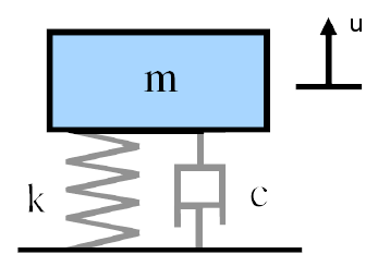
对于图 1 所示的简单质量-弹簧-阻尼器系统,其运动方程为 —
\begin{align} \label{eq:14801a} F(t) &= m \, \frac{d^2u}{dt^2} + c \, \frac{du}{dt} + k \, u \\[0.7em]%eqn_interline_spacing &= m \, \ddot{u} + c \, \dot{u} + k \, u \nonumber \end{align}
式中 —
| \( F(t) \) | = 激励函数 |
| \( u \) | = 位移 |
| \( \frac{du}{dt} \) | = 速度(\(\dot{u}\)) |
| \( \frac{d^2u}{dt^2} \) | = 加速度(\(\ddot{u}\)) |
| \( m \) | = 质量 |
| \( c \) | = 阻尼常数(粘性) |
| \( k \) | = 弹簧刚度 |
注:在机械系统中可能存在多种阻尼。上述方程假设为粘性阻尼,即阻尼力与速度成正比。
运动质量因其速度而储存的能量为 —
\begin{align} \label{eq:14802a} W_m = \frac{1}{2} \, m \, \dot{u}^2 \end{align}
弹簧因其拉伸而储存的能量为 —
\begin{align} \label{eq:14803a} W_k = \frac{1}{2} \, k \, u^2 \end{align}
阻尼器耗散的功率为 —
\begin{align} \label{eq:14804a} P_c = c \, \dot{u}^2 \end{align}
谐振频率为 —
\begin{align} \label{eq:14805a} f = \sqrt\frac{k}{m} \end{align}
电振荡
|
|
|
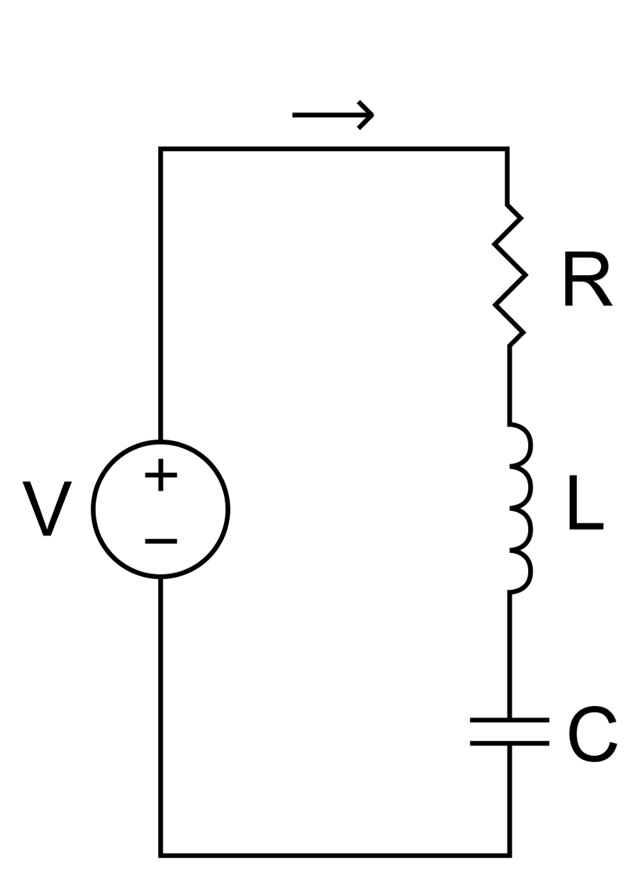
对于图 2 所示的简单电感-电容-电阻电路,其电路方程为 —
\begin{align} \label{eq:14820a} V(t) &= L \, \frac{d^2q}{dt^2} + R \, \frac{dq}{dt} + \frac{1}{C} \, q \\[0.7em]%eqn_interline_spacing &= L \, \ddot{q} + R \, \dot{q} + \frac{1}{C} \, q \nonumber \end{align}
式中 —
| \( V(t) \) | = 电压函数 |
| \( q \) | = 电荷 |
| \( \frac{dq}{dt} \) | = 电流(\(\dot{q}\)) |
| \( \frac{d^2q}{dt^2} \) | = zzz(\(\ddot{q}\)) |
| \( L \) | = 电感 |
| \( R \) | = 电阻 |
| \( C \) | = 电容 |
电感因电荷运动而储存的能量为 —
\begin{align} \label{eq:14851a} W_L = \frac{1}{2} \, L \, \dot{q}^2 \end{align}
电容因储存电荷而储存的能量为 —
\begin{align} \label{eq:14852a} W_C = \frac{1}{2} \, \frac{1}{C} \, q^2 \end{align}
电阻耗散的功率为 —
\begin{align} \label{eq:14853a} P_R = R \, \dot{q}^2 \end{align}
谐振频率为 —
\begin{align} \label{eq:14854a} f = \sqrt\frac{1}{L \, C} \end{align}
对比
对比相应的机械方程与电学方程,可以明显看出以下类比关系。这些类比在讨论换能器等效电路时特别有用。
|
||||||||||||||
|
注意,机械刚度 \( k \) 的类比量是电容的倒数 \( 1/C \)。因此,增大电容会降低刚度。所以电容也类比于机械柔度。
Mechanical—Electrical analogs
Systems that oscillate mechanically or electrically have similar characteristics. This page will establish the mechanical-electrical analogs.
Mechanical oscillation
|
|
|
For the simple mass-spring-damper system of figure 1, the equation of motion is —
\begin{align} \label{eq:14801a} F(t) &= m \, \frac{d^2u}{dt^2} + c \, \frac{du}{dt} + k \, u \\[0.7em]%eqn_interline_spacing &= m \, \ddot{u} + c \, \dot{u} + k \, u \nonumber \end{align}
where —
| \( F(t) \) | = forcing function |
| \( u \) | = displacement |
| \( \frac{du}{dt} \) | = velocity (\(\dot{u}\)) |
| \( \frac{d^2u}{dt^2} \) | = acceleration (\(\ddot{u}\)) |
| \( m \) | = mass |
| \( c \) | = damping constant (viscous) |
| \( k \) | = spring stiffness |
Note: in mechanical systems various kinds of damping are possible. The above equation assumes viscous damping where the damping force is proportional to the velocity.
The energy stored in the moving mass due to its velocity is —
\begin{align} \label{eq:14802a} W_m = \frac{1}{2} \, m \, \dot{u}^2 \end{align}
The energy stored in the spring due to its stretch is —
\begin{align} \label{eq:14803a} W_k = \frac{1}{2} \, k \, u^2 \end{align}
The power dissipated by the damper is —
\begin{align} \label{eq:14804a} P_c = c \, \dot{u}^2 \end{align}
The resonant frequency is —
\begin{align} \label{eq:14805a} f = \sqrt\frac{k}{m} \end{align}
Electrical oscillation
|
|
|
For the simple inductor-capacitor-resistor circuit of figure 2, the circuit equation is —
\begin{align} \label{eq:14820a} V(t) &= L \, \frac{d^2q}{dt^2} + R \, \frac{dq}{dt} + \frac{1}{C} \, q \\[0.7em]%eqn_interline_spacing &= L \, \ddot{q} + R \, \dot{q} + \frac{1}{C} \, q \nonumber \end{align}
where —
| \( V(t) \) | = voltage function |
| \( q \) | = charge |
| \( \frac{dq}{dt} \) | = current (\(\dot{q}\)) |
| \( \frac{d^2q}{dt^2} \) | = zzz (\(\ddot{q}\)) |
| \( L \) | = inductance |
| \( R \) | = resistance |
| \( C \) | = capacitance |
The energy stored in the inductor due to the moving charge is —
\begin{align} \label{eq:14851a} W_L = \frac{1}{2} \, L \, \dot{q}^2 \end{align}
The energy stored in the capacitor due to the stored charge is —
\begin{align} \label{eq:14852a} W_C = \frac{1}{2} \, \frac{1}{C} \, q^2 \end{align}
The power dissipated by the resistor is —
\begin{align} \label{eq:14853a} P_R = R \, \dot{q}^2 \end{align}
The resonant frequency is —
\begin{align} \label{eq:14854a} f = \sqrt\frac{1}{L \, C} \end{align}
Comparison
Comparing the corresponding mechanical and electrical equations, the following analogs are apparent. These analogs are particularly useful in discussing transducer equivalent circuits.
|
||||||||||||||
|
Note that the analog of the mechanical stiffness \( k \) is the reciprocal of the electrical capacitance \( 1/C \). Thus, increasing the capacitance reduces the stiffness. Hence the capacitance is also analagous to mechanical compliance.