空化
空化是指液体内含有蒸气或蒸气与气体混合物的空穴或气泡的形成及随后的溃灭(ASTM-G32)。在超声场的作用下,这种生长和溃灭通常在少数几个超声周期内发生。这些气泡的溃灭会在局部产生极高的压力和温度。
估算功率(水)
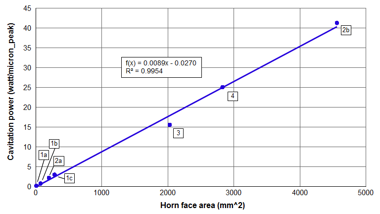
对于端面为圆形的变幅杆,其在室温脱气水中的空化功率可以从下图估算。
|
|
|
|
||||||||||||||||||||||||||||||||
|
说明 —
- 方法 1 = 用功率计测量净功率。传递给流体的净空化功率等于空化期间换能器的总输入功率减去超声叠堆中的功率损耗。作为近似,超声叠堆的损耗取为超声叠堆的空载功率(即在空气中运行时的功率)。然而,已知换能器压电陶瓷耗散的功率随输出功率的增大而增大,因此用空载近似估算叠堆损耗会偏低。于是,计算出的净空化功率会有些偏高。输出功率越大,误差越大。不过,误差应该不会很大。
- 方法 2 = 量热法。在规定的时间内测量水的温升。由此可以根据水的比热和体积计算出空化功率。
- Peshkovsky 的数据是在 17.8 kHz 下测得的。为了与其他数据保持一致,Peshkovsky 的数据被外推到 20 kHz,其假设是单位振幅的功率随频率线性增加(即无论频率如何,单位速度的功率恒定)。该假设尚待验证。
- 如果变幅杆的端面振幅不完全均匀,则应使用变幅杆端面振幅的平均值来由图 1 计算功率(因为空化功率随振幅线性变化)。
- 虽然图 1 的数据是针对圆柱形变幅杆测得的,但只要变幅杆的厚度与宽度大致相当,回归方程可能也近似适用于矩形变幅杆。
空化强度可以从曲线图的斜率得出 — 即 0.89 瓦/微米_峰值/cm²。
空化受众多参数影响。流体性质包括蒸气压、表面张力、粘度和密度。外部因素包括温度、空化核的数量(悬浮颗粒和溶解气体)以及流体容器的形状和距离。因此,图 1 只应作为预期空化功率的粗略估计。如果流体不是水,则图 1 不适用。
示例
假设有一个 20 kHz Ø50 mm 的变幅杆,端面振幅为 50 微米_峰值。(在此直径下端面振幅接近均匀,因此无需对端面振幅取平均。)
变幅杆的端面面积为 1963 mm2。由图 1 的方程,空化功率为 17.4 瓦/微米_峰值。那么在 50 微米_峰值下,估算的空化功率为 870 瓦(向上取整为 900 瓦)。这仅仅是净空化功率。驱动超声叠堆还需要额外的功率。
温度的影响
上述数据针对的是室温(25°C)下的水。然而,随着温度升高,给定振幅下的空化功率会下降。例如,关于水的数据见 Raso[1] 和 Löning[1],关于各种油类的数据见 Kobus[2]。
振幅的影响
人们可能以为空化功率会随振幅的平方变化(类似于电阻的 \( I^2 R \) 定律)。如果空化电阻与输入振幅无关,情况确实会如此。然而事实上,空化气泡云的电阻随振幅变化。随着振幅增大,变幅杆端面处的气泡数量也会增加;于是,更厚的气泡云减弱了变幅杆与液体之间的耦合,使能量传递变得相对更加困难。
下图取自 Peshkovsky[1](图 9,第 321 页),表明在给定频率下,空化功率随变幅杆端面速度(因而也随振幅)线性变化。Peshkovsky 的频率为 17.8 kHz。注意,Peshkovsky 的速度是 RMS(均方根;将 \( V_{RMS} \) 乘以 \( \sqrt{2} \) 即可换算为峰值速度)。
|
|
|
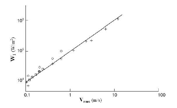
注:除圈出的数据在 2 bar 压力下测得外,所有数据均在 1 bar [1 个大气压 = 0.1 MPa] 下测得。
图 2 中直线的方程为(Peshkovsky,第 321 页)—
\begin{align} \label{eq:14601a} W_1 &= P_0 \, V_{RMS} \end{align}
其中 —
| \( P_0 \) | = 静压力 [Pa] |
频率的影响
随着频率升高,相邻超声周期之间的时间缩短。因此,空化气泡在溃灭前生长的时间更少。于是,更高的频率会产生更小的气泡,每个气泡所含的能量也更少。(作为一阶近似,气泡半径与频率成反比。见 Leighton[1],公式 11.1,第 200 页;另见 Piazza[1],公式 1,第 3 页。)另一方面,更高的频率意味着单位时间内有更多的气泡溃灭(对于给定数量的气泡),也可能导致更大的气泡密度(单位体积流体中的气泡数)。对功率的净影响是……?
应用
上述关于功率的讨论多少带有学术性质,因为实际应用很少在室温水中进行。功率还受其他因素影响,包括流体粘度、表面张力和颗粒浓度。
Cavitation
Cavitation is the formation and subsequent collapse, within a liquid, of cavities or bubbles that contain vapor or a mixture of vapor and gas (ASTM-G32). In the presence of an ultrasonic field, this growth and collapse typically occurs during a small number of ultrasonic cycles. The collapse of these bubbles causes locally intense pressures and temperatures.
Estimated power (water)
For a horn with a circular face, the cavitation power in degassed water at room temperature can be estimated from the following graph.
|
|
|
|
||||||||||||||||||||||||||||||||
|
Notes —
- Method 1 = Wattmeter measuring net power. The net cavitation power to the fluid is the total input power to the transducer during cavitation minus the power loss in the ultrasonic stack. As an approximation, the loss in the ultrasonic stack is taken as the no-load power of the ultrasonic stack (i.e., the power when running in air). However, it is known that the power dissipated by the transducer's ceramics increases as the delivered power increases so the no-load approximation of stack loss is too low. Hence, the calculated net cavitation power will be somewhat too high. The error increases as the delivered power increases. However, the error should not be large.
- Method 2 = Calorimetric. The temperature rise of the water is measured over a specified time. From this the cavitation power can be calculated based on the water's specific heat and volume.
- Peshkovsky's data was measured at 17.8 kHz. In order to be consistent with the other data, Peshkovsky's data has been extrapolated to 20 kHz under the assumption that the power per unit amplitude increases linearly with frequency (i.e., the power per unit velocity is constant, regardless of frequency). This assumption awaits verification.
- If the horn's face amplitude is not completely uniform then the horn's average face amplitude should be used to calculate the power from figure 1 (since the cavitation power varies linearly with amplitude).
- Although the data from figure 1 were taken for cylindrical horns, the regression equation would likely apply approximately for rectangular horns provided that the horn's thickness is somewhat comparable to the width.
The cavitation intensity can be taken from the slope of the graph — i.e., 0.89 watt/micron_peak/cm².
Cavitation is affected by numerous parameters. Fluid properties include vapor pressure, surface tension, viscosity, and density. External factors include temperature, the number of cavitation nuclei (suspended particlas and dissolved gasses), and the shape and proximity of the fluid container. Thus, figure 1 should only be used as a rough estimate of the expected cavitation power. If the fluid is not water then figure 1 would not apply.
Example
Assume a 20 kHz Ø50 mm horn with a face amplitude of 50 microns_peak. (At this diameter the face amplitude is nearly uniform so no averaging of the face amplitude is needed.)
The horn's face area is 1963 mm2. From the equation from figure 1, the cavitation power is 17.4 watt/micron_peak. Then at 50 microns_peak the estimated cavitation power is 870 watts (round up to 900 watts). This is the net cavitation power alone. Additional power would be needed to drive the ultrasonic stack.
Effect of temperature
The above data are for water at room temperature (25°C). However, as the temperature increases the cavitation power at a given amplitude decreases. For example, see Raso[1] and Löning[1] for water and Kobus[2] for various oils.
Effect of amplitude
One might expect that cavitation power would vary with the square of the amplitude (similar to the \( I^2 R \) law for a resistor). This would be true if the cavitation resistance were independent of input amplitude. In fact, however, the resistance of the cavitating bubble cloud is not constant with amplitude. As the amplitude increases the number of bubbles at the face of the horn also increases; thus, the coupling of the horn to the liquid is reduced by the thicker bubble cloud so that the transfer of energy becomes relatively more difficult.
The following figure from Peshkovsky[1] (figure 9, p. 321) shows that cavitation power varies linearly with the horn's face velocity (and hence with amplitude) at a given frequency. Peshkovsky's frequency was 17.8 kHz. Note that Peshkovsky's velocity is RMS (root mean squared; multiply \( V_{RMS} \) by \( \sqrt{2} \) to convert to peak velocity).
|
|
|
Note: All data are at 1 bar [1 atmosphere = 0.1 MPa] except the circled data which are at 2 bars of pressure.
The equation of the line in figure 2 is (Peshkovsky, p. 321) —
\begin{align} \label{eq:14601a} W_1 &= P_0 \, V_{RMS} \end{align}
where —
| \( P_0 \) | = Static pressure [Pa] |
Effect of frequency
As the frequency increases, the time between successive ultrasonic cycles decreases. Therefore, the cavitation bubble has less time to grow before it collapses. Hence, higher frequencies result in smaller bubbles, each of which contains less energy. (As a first approximation, the bubble radius is inversely proportional to the frequency. See Leighton[1], eq. 11.1, p. 200; also, Piazza[1], eq. 1, p. 3.) On the other hand, higher frequencies yield more bubble collapses per unit time (for a give number of bubbles) and may may also result in greater bubble densities (bubbles per unit volume of fluid). The net effect on power is ... ?
Application
The above discussion of power is somewhat academic since applications are seldom conducted in room temperature water. Power is affected by additional factors including fluid viscosity, surface tension, and particulate concentration.