附录 H — 叠堆螺栓对机电耦合系数 κ 的影响
当陶瓷由叠堆螺栓施加预应力时,机电耦合系数 \( kappa \) 会降低,因为叠堆螺栓的刚度会抑制陶瓷的正常膨胀或收缩。本附录推导这一关系。(注:在本讨论中,"叠堆螺栓"指对陶瓷叠堆施加预应力的任何手段,包括中心叠堆螺栓、周边叠堆螺栓或周边壳体。)
一般性讨论见换能器设计 — 叠堆螺栓。
考虑由 \( n \) 片相同介电陶瓷组成的叠堆,夹在两块平行的刚性无质量压板之间。当对每片陶瓷施加直流电压 \( V \) 时,能量传递到陶瓷为其电容充电。总"电容能量"为 —
\begin{align} \label{eq:10028a} \widehat{W}_c &= n \, \left( \small\frac{1}{2} \, C \, V^2 \right) \end{align}
其中 —
| \( \widehat{W}_c \) | = 电容能量 [库仑-伏特或焦耳] |
| \( C \) | = 单片陶瓷的电容 [库仑/伏特或法拉] |
| \( V \) | = 电压 [伏特] |
| \( n \) | = 陶瓷片数 |
如果陶瓷还具有压电特性,则会传递额外的能量,使陶瓷膨胀或收缩;这正是将所施加电能转化为机械(应变)能的期望效应。该应变能为 —
\begin{align} \label{eq:10027a} \widehat{W}_k &= \small\frac{1}{2} \, k \, U^2 \end{align}
其中 —
| \( \widehat{W}_k \) | = 应变能 [N-m 或焦耳] |
| \( k \) | = 陶瓷叠堆的刚度 [N/m] |
| \( U \) | = 电压 \( V \) [m] 引起的陶瓷叠堆位移 |
如果存在叠堆螺栓且同样连接在两块压板之间,则刚度 \( k \) 包含陶瓷 \( k_c \) 与叠堆螺栓 \( k_s \) 的组合刚度。
机电耦合系数 \( \kappa \)(kappa)由 Waanders (1) 第 12 页给出为 —
\begin{align} \label{eq:10026a} \kappa^2 &= {\left[\frac{\textsf{Energy converted}}{\textsf{Energy input}} \right]}_{\textsf {Low frequency}} \end{align}
注意"低频"的要求,即测量频率远低于器件的谐振频率。在此条件下,速度引起的惯性能量与变形引起的应变能相比可以忽略。由于 \( \kappa \) 是两个能量之比,\( \kappa \) 必定是无量纲的。
在陶瓷叠堆由外加电压激励的情形下,"Energy converted" (被转换的能量)是从电的形式转换为机械形式的能量。因此,方程 \eqref{eq:10026a} 的分子正是方程 \eqref{eq:10027a} 的应变能 \( \widehat{W}_k \)。分母是总输入(系统)能量(即 \( \widehat{W}_c \) 与 \( \widehat{W}_k \) 的能量之和)。于是,方程 \eqref{eq:10026a} 可写为 —
\begin{align} \label{eq:10029a} \kappa^2 &=\cfrac{\widehat{W}_k}{\widehat{W}_c + \widehat{W}_k} \\[0.7em]%complex_eqn_interline_spacing &= \cfrac{1}{\left( \cfrac{\widehat{W}_c}{\widehat{W}_k} \right) +1} \nonumber \\[0.7em]%complex_eqn_interline_spacing &= \cfrac{1}{\left( \cfrac{n \, C}{k} \right) {\left( \cfrac{V}{U} \right)}^2 +1} \nonumber \end{align}
方程 \eqref{eq:10029a} 是完全通用的。下面将其分别应用于无叠堆螺栓(情形 1)和有叠堆螺栓(情形 2)的情况。
情形 1 — 无叠堆螺栓
在方程 \eqref{eq:10029a} 中赋予下标 1,以表示无叠堆螺栓 —
\begin{align} \label{eq:10030a} {\kappa_1}^2 &= \frac{1}{{\left(\Large\frac{n \, C}{k_1}\right) } \left(\Large\frac{V}{U_1} \right)^2 +1} \end{align}
由于没有叠堆螺栓,这里的 \( k_1 \) 仅为陶瓷叠堆自身的刚度。为方便起见,将其记为 \( k_c \)。
求解 \( \left(\frac{V}{U_1}\right)^2 \)(供后面使用)—
\begin{align} \label{eq:10031a} \left(\frac{V}{U_1} \right)^2= \frac{\Large{\frac{1}{{\kappa_1}^2}} -1}{\left(\Large\frac{n \, C}{k_c}\right) } \end{align}
\( \kappa \) 对试验参数的依赖关系
看起来方程 \eqref{eq:10030a} 给出的 \( \kappa \) 似乎取决于特定的试验参数(例如 \( C \) 和 \( k_c \),二者都取决于陶瓷尺寸,还有 \( n \)、\( V \) 和 \( U \))。然而实际上,\( \kappa \) 只取决于陶瓷的机电特性,如下所证。
考察方程 \eqref{eq:10030a} 中的各参数与陶瓷尺寸的关系(由此得到下面的方程 \eqref{eq:10031b}、\eqref{eq:10031c} 和 \eqref{eq:10031d})。
考察 \( C \) —
\begin{align} \label{eq:10031b} C &= {\frac{\varepsilon \, A_c}{h_c}} \end{align}
其中 —
| \( \varepsilon \) | = 陶瓷介电常数 [(库仑/伏特)/m] |
| \( A_c \) | = 陶瓷的横截面积(即单片陶瓷平面的面积)[m²] |
| \( h_c \) | = 每片陶瓷的高度(厚度)[m] |
考察 \( k_c \) —
\begin{align} \label{eq:10031c} k_c &= {\left( \frac{1}{n} \right) \left( \frac{Y_c \, A_c}{h_c}\right)} \end{align}
其中 —
| \( Y_c \) | = 陶瓷的杨氏模量 |
考察 \( \frac{V}{U_1} \) —
\begin{align} \label{eq:10031d} \frac{V}{U_1} &= \frac{V / h_c}{U_1 / h_c} \\[0.7em]%complex_eqn_interline_spacing &= \frac{V / h_c}{n \, \left[ \left(U_1/n \right) / h_c \right]} \nonumber \\[0.7em]%complex_eqn_interline_spacing &= \frac{E}{n \, \epsilon} \nonumber \\[0.7em]%complex_eqn_interline_spacing &= \frac{1}{n \, (\epsilon / E)} \nonumber \\[0.7em]%complex_eqn_interline_spacing &= \frac{1}{n \, d_{33}} \nonumber \end{align}
其中 —
| \( E \) | = 电场强度 [v/m] |
| \( \epsilon \) | = 每片陶瓷中的应变 [v/m] |
| \( d_{33} \) | = 压电应变常数 [m/v] 或电荷常数 [Coulonb/N] |
在方程 \eqref{eq:10031d} 中,注意 \( U_1 \) 是所有陶瓷(即整个陶瓷叠堆)的总位移。因此,\( U_1/n \) 是单片陶瓷的位移,\( (U_1/n)/h_c \) 便是单片陶瓷中的应变 \( \epsilon \)。于是,该应变 \( \epsilon \) 除以电场强度 \( E \) 正是压电应变常数 \( d_{33} \)。
现在,将方程 \eqref{eq:10031b}、\eqref{eq:10031c} 和 \eqref{eq:10031d} 代入 \eqref{eq:10030a},得到 —
\begin{align} \label{eq:10031e} {\kappa_1}^2 &= \frac{1}{{\left(\Large\frac{\varepsilon}{Y}\right) } \left(\Large\frac{1}{d_{33}} \right)^2 +1} \end{align}
因此,当无螺栓时,机电耦合 \( \kappa_1 \) 只取决于陶瓷的特性,而与陶瓷片数或试验的其他参数无关。不过应当注意,陶瓷的某些"特性"取决于电学和力学边界条件。
如上所述,机电耦合系数 \( \kappa \) 是能量之比,因此应是无量纲的。于是 \eqref{eq:10031e} 的右边也应是无量纲的。对 \eqref{eq:10031e} 分母中的变量进行量纲分析,得到 —
\begin{align} \label{eq:10031f} \left( \frac {\left( \frac{coulomb/volt}{m} \right)} {\left( \frac{N}{m^2} \right)} \right) \left(\frac{1}{volt/m} \right)^2 = \frac{coulomb \, volt}{N \, m} = \frac{joule}{joule} = dimensionless \end{align}
情形 2 — 有叠堆螺栓
在方程 \eqref{eq:10029a} 中赋予下标 2,以表示有叠堆螺栓 —
\begin{align} \label{eq:10032a} {\kappa_2}^2 &= \frac{1}{{\left(\Large\frac{C}{k_2}\right) } \left(\Large\frac{V}{U_2} \right)^2 +1} \\[0.7em]%complex_eqn_interline_spacing &= \frac{1}{{\left(\Large\frac{C}{k_2}\right) } \left(\Large\frac{V}{U_1} \right)^2 \left(\Large\frac{U_1}{U_2} \right)^2 +1} \nonumber \end{align}
\( k_2 \) 是叠堆总刚度。由于陶瓷与螺栓在力学上是并联的,\( k_2 \) 就等于陶瓷刚度加上螺栓刚度 —
\begin{align} \label{eq:10032b} k_2 = k_c + k_b \end{align}
其中 —
| \( k_2 \) | = 叠堆总刚度 [N/m] |
| \( k_c \) | = 陶瓷总刚度 [N/m] |
| \( k_b \) | = 螺栓轴向刚度 [N/m] |
于是方程 \eqref{eq:10032a} 变为 —
\begin{align} \label{eq:10032c} {\kappa_2}^2 &= \frac{1}{{\left(\Large\frac{C}{k_c \, + \, k_b}\right) } \left(\Large\frac{V}{U_1} \right)^2 \left(\Large\frac{U_1}{U_2} \right)^2 +1} \end{align}
对于给定的陶瓷构型,叠堆位移 \( U \) 与叠堆刚度成反比。因此,一般有 —
\begin{align} \label{eq:10033a} U \,\propto \, \frac{1}{k} \end{align}
于是,无叠堆螺栓时的相对位移 \( U_1 \) 与有叠堆螺栓时的相对位移 \( U_2 \) 可用刚度表示为 —
\begin{align} \label{eq:10034a} \frac{U_1}{U_2} &= \frac{k_2}{k_1} \\[0.7em]%complex_eqn_interline_spacing &= \frac{k_c \, + \, k_b}{k_c} \nonumber \\[0.7em]%complex_eqn_interline_spacing &= \frac{k_b}{k_c} + 1 \nonumber \end{align}
将方程 \eqref{eq:10031a} 和 \eqref{eq:10034a} 代入方程 \eqref{eq:10032c} 并化简,得到 —
\begin{align} \label{eq:10037a} {\kappa_2}^2 &= \frac{1}{ \left({\Large\frac{1}{{\kappa_1}^2}} -1 \right) \left({\Large\frac{k_b}{k_c}} +1\right) +1} \end{align}
其中(最终)—
| \( \kappa_2 \) | = 有叠堆螺栓时的压电耦合系数 |
| \( \kappa_1 \) | = 无叠堆螺栓时的压电耦合系数 |
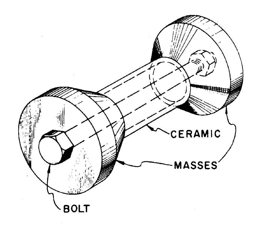
Berlincourt[3](第 269 页尾注 9,在第 249 页被引用)针对重质量负载换能器给出了相同的方程,只是记号略有不同并做了一些整理。(理想的重质量负载换能器是指陶瓷居中、且陶瓷体积与两个端部质量块相比很小的换能器,两个端部质量块被假定为无限刚性(即无应变)。于是当换能器在谐振状态振动时,陶瓷和叠堆螺栓承受近乎均匀的应变。这种均匀应变与此处对静态加载所作的假定相同。)
|
|
|
如果没有螺栓(即 \( k_b = 0 \)),则 \( \kappa_2 = \kappa_1 \),与预期一致。随着螺栓刚度 \( k_b \) 增大,\( \kappa_2 \) 逐渐降低到 \( \kappa_1 \) 以下。 如果螺栓刚度 \( k_b \) (理论上)变为无穷大,则 \( \kappa_2 \) 为零。这是因为无论施加多大电压,叠堆都被螺栓约束而无法产生任何膨胀。于是,所有外加电压都用于给陶瓷充电,而不会引起陶瓷的任何膨胀。
对于陶瓷叠堆的每个组成部分,刚度可用该部分的模量和尺寸表示 —
\begin{align} \label{eq:10038a} k &= Y A / h \end{align}
其中 —
| \( Y \) | = 杨氏模量 |
| \( A \) | = 横截面积 |
| \( h \) | = 部件的高度(长度) |
因此,用实际的陶瓷和螺栓参数表示,方程 \eqref{eq:10037a} 可写为 —
\begin{align} \label{eq:10039a} {\kappa_2}^2 &= \frac{1}{ \left({\Large\frac{1}{{\kappa_1}^2}} -1 \right) \left({\Large\frac{Y_b \, A_b \, / \, h_b}{Y_c \, A_c \,/ \, (n \, h_c)}} +1\right) +1} \end{align}
其中 —
| \( Y_b \) | = 螺栓的杨氏模量 |
| \( A_b \) | = 螺栓杆部的横截面积 |
| \( h_b \) | = 螺栓的长度 |
| \( Y_c \) | = 陶瓷的杨氏模量 |
| \( A_c \) | = 陶瓷的横截面积(即单片陶瓷平面的面积) |
| \( h_c \) | = 单片陶瓷的高度(厚度) |
| \( n \) | = 陶瓷片数 |
注意,\( n \, h_c \) 就是陶瓷叠堆的总高度。还应注意,\( h_b \) 可以长于 \( n \, h_c \),这并不违反上述推导的前提条件。
Appendix H — Effect of stack bolt on electromechanical coupling coefficient κ
When the ceramics are prestressed by a stack bolt, the electromechanical coupling coefficient \( kappa \) is reduced because the stiffness of the stack bolt reduces the normal expansion or contraction of the ceramics. This appendix derives the relationship. (Note: in this discussion, "stack bolt" refers to any means of applying a prestress to the ceramic stack. This could include a center stack bolt, peripheral stack bolts, or a peripheral shell.)
See Transducer design — stack bolt for a general discussion.
Consider a stack of \( n \) identical dielectric ceramics that are contained between two parallel rigid massless platens. When a D-C voltage \( V \) is applied to each ceramic, energy is transferred to the ceramics to charge the ceramic's capacitance. The total "capacitive energy" is —
\begin{align} \label{eq:10028a} \widehat{W}_c &= n \, \left( \small\frac{1}{2} \, C \, V^2 \right) \end{align}
where —
| \( \widehat{W}_c \) | = capacitive energy [coulomb-volt or joules] |
| \( C \) | = ceramic individual capacitance [coulomb/volt or farads] |
| \( V \) | = voltage [volts] |
| \( n \) | = number of ceramics |
If the ceramics also have piezoelectric properties then additional energy is transferred which causes the ceramic to expand or contract; this is the desired effect by which the applied electrical energy is transformed into mechanical (strain) energy. This strain energy is —
\begin{align} \label{eq:10027a} \widehat{W}_k &= \small\frac{1}{2} \, k \, U^2 \end{align}
where —
| \( \widehat{W}_k \) | = strain energy [N-m or joules] |
| \( k \) | = stiffness of ceramic stack [N/m] |
| \( U \) | = displacement of ceramic stack due to voltage \( V \) [m] |
If a stack bolt is present and is also connected between the two platens then the stiffness \( k \) includes the combined stiffness of the ceramics \( k_c \) and the stack bolt \( k_s \).
The electromechanical coupling coefficient \( \kappa \) (kappa) is given by Waanders (1), p. 12 as —
\begin{align} \label{eq:10026a} \kappa^2 &= {\left[\frac{\textsf{Energy converted}}{\textsf{Energy input}} \right]}_{\textsf {Low frequency}} \end{align}
Note the requirement of "low frequency" for which the measurement frequency is well below the resonant frequency of the device. Under this condition the inertial energy due to velocity is negligible compared to the strain energy due to deformation. Since \( \kappa \) is the ratio of two energies, \( \kappa \) must be dimensionless.
In the case where the ceramic stack is excited by an applied voltage, the "Energy converted" is the energy that is converted from electrical form to mechanical form. Hence, the numerator of equation \eqref{eq:10026a} is just the strain energy \( \widehat{W}_k \) of equation \eqref{eq:10027a}. The denomintor is the total input (system) energy (i.e., the combined energy of \( \widehat{W}_c \) and \( \widehat{W}_k \)). Thus, equation \eqref{eq:10026a} can be written as —
\begin{align} \label{eq:10029a} \kappa^2 &=\cfrac{\widehat{W}_k}{\widehat{W}_c + \widehat{W}_k} \\[0.7em]%complex_eqn_interline_spacing &= \cfrac{1}{\left( \cfrac{\widehat{W}_c}{\widehat{W}_k} \right) +1} \nonumber \\[0.7em]%complex_eqn_interline_spacing &= \cfrac{1}{\left( \cfrac{n \, C}{k} \right) {\left( \cfrac{V}{U} \right)}^2 +1} \nonumber \end{align}
Equation \eqref{eq:10029a} is perfectly general. It will be applied below when there is no stack bolt (case 1) and when a stack bolt is present (case 2).
Case 1 — no stack bolt
Assigning subscript 1 in equation \eqref{eq:10029a} to indicate that no stack bolt is present —
\begin{align} \label{eq:10030a} {\kappa_1}^2 &= \frac{1}{{\left(\Large\frac{n \, C}{k_1}\right) } \left(\Large\frac{V}{U_1} \right)^2 +1} \end{align}
Here \( k_1 \) is the stiffness of ceramic stack alone since there is no stack bolt. For convenience we designate this as \( k_c \).
Solving for \( \left(\frac{V}{U_1}\right)^2 \) (for later use) —
\begin{align} \label{eq:10031a} \left(\frac{V}{U_1} \right)^2= \frac{\Large{\frac{1}{{\kappa_1}^2}} -1}{\left(\Large\frac{n \, C}{k_c}\right) } \end{align}
Dependence of \( \kappa \) on test parameters
It might appear that \( \kappa \) given in equation \eqref{eq:10030a} depends on the particular test parameters (e.g., \( C \) and \( k_c \) which both depend on the ceramic dimensions, and also \( n \), \( V \) and \( U \)). In fact, however, \( \kappa \) depends only on the electromechanical properties of the ceramic, as demonstrated below.
Consider how the parameters in equation \eqref{eq:10030a} are related to the ceramic dimensions (resulting in equations \eqref{eq:10031b}, \eqref{eq:10031c}, and \eqref{eq:10031d} below).
Consider \( C \) —
\begin{align} \label{eq:10031b} C &= {\frac{\varepsilon \, A_c}{h_c}} \end{align}
where —
| \( \varepsilon \) | = ceramic permittivity [(coulomb/volt)/m] |
| \( A_c \) | = cross-sectional area of ceramic (i.e., the area of the individual ceramic's flat face) [m²] |
| \( h_c \) | = height (thickness) of each ceramic [m] |
Consider \( k_c \) —
\begin{align} \label{eq:10031c} k_c &= {\left( \frac{1}{n} \right) \left( \frac{Y_c \, A_c}{h_c}\right)} \end{align}
where —
| \( Y_c \) | = Young's modulus of the ceramic |
Consider \( \frac{V}{U_1} \) —
\begin{align} \label{eq:10031d} \frac{V}{U_1} &= \frac{V / h_c}{U_1 / h_c} \\[0.7em]%complex_eqn_interline_spacing &= \frac{V / h_c}{n \, \left[ \left(U_1/n \right) / h_c \right]} \nonumber \\[0.7em]%complex_eqn_interline_spacing &= \frac{E}{n \, \epsilon} \nonumber \\[0.7em]%complex_eqn_interline_spacing &= \frac{1}{n \, (\epsilon / E)} \nonumber \\[0.7em]%complex_eqn_interline_spacing &= \frac{1}{n \, d_{33}} \nonumber \end{align}
where —
| \( E \) | = electric field strength [v/m] |
| \( \epsilon \) | = strain in each ceramic [v/m] |
| \( d_{33} \) | = piezoelectric strain constant [m/v] or charge constant [Coulonb/N] |
In equation \eqref{eq:10031d}, note that \( U_1 \) is the combined desplacement of all of the ceramics (i.e., the entire ceramic stack). Therefore, \( U_1/n \) is the displacement of a single ceramic so \( (U_1/n)/h_c \) is the strain \( \epsilon \) in a single ceramic. Then that strain \( \epsilon \) divided by the electric field strength \( E \) is just the piezoelectric strain constant \( d_{33} \).
Now, substituting equations \eqref{eq:10031b}, \eqref{eq:10031c}, and \eqref{eq:10031d} into \eqref{eq:10030a} gives —
\begin{align} \label{eq:10031e} {\kappa_1}^2 &= \frac{1}{{\left(\Large\frac{\varepsilon}{Y}\right) } \left(\Large\frac{1}{d_{33}} \right)^2 +1} \end{align}
Thus, when no bolt is present the electromagnetic coupling \( \kappa_1 \) depends only on properties of the ceramic, not on the number of ceramics or other parameters of the test. It should be noted, however, that some of the ceramic "properties" depend on the electrical and mechanical boundary conditions.
As discussed above, the electromechanical coupling factor \( \kappa \) is the ratio of energies and so should be dimensionless. Thus, the right side of \eqref{eq:10031e} should also be dimensionless. Performing a dimensional analysis on the variables in the denominator of \eqref{eq:10031e} gives —
\begin{align} \label{eq:10031f} \left( \frac {\left( \frac{coulomb/volt}{m} \right)} {\left( \frac{N}{m^2} \right)} \right) \left(\frac{1}{volt/m} \right)^2 = \frac{coulomb \, volt}{N \, m} = \frac{joule}{joule} = dimensionless \end{align}
Case 2 — with stack bolt
Assigning subscript 2 in equation \eqref{eq:10029a} to indicate that a stack bolt is present —
\begin{align} \label{eq:10032a} {\kappa_2}^2 &= \frac{1}{{\left(\Large\frac{C}{k_2}\right) } \left(\Large\frac{V}{U_2} \right)^2 +1} \\[0.7em]%complex_eqn_interline_spacing &= \frac{1}{{\left(\Large\frac{C}{k_2}\right) } \left(\Large\frac{V}{U_1} \right)^2 \left(\Large\frac{U_1}{U_2} \right)^2 +1} \nonumber \end{align}
\( k_2 \) is the total stack stiffness. Since the ceramics and bolt are mechanically in parallel, the \( k_2 \) just equals the ceramic stiffness plus the bolt stiffness —
\begin{align} \label{eq:10032b} k_2 = k_c + k_b \end{align}
where —
| \( k_2 \) | = total stack stiffness [N/m] |
| \( k_c \) | = total ceramic stiffness [N/m] |
| \( k_b \) | = bolt axial stiffness [N/m] |
Thus equation \eqref{eq:10032a} becomes —
\begin{align} \label{eq:10032c} {\kappa_2}^2 &= \frac{1}{{\left(\Large\frac{C}{k_c \, + \, k_b}\right) } \left(\Large\frac{V}{U_1} \right)^2 \left(\Large\frac{U_1}{U_2} \right)^2 +1} \end{align}
For a given ceramic configuration the stack displacement \( U \) varies inversely with the stack stiffness. Thus, generally —
\begin{align} \label{eq:10033a} U \,\propto \, \frac{1}{k} \end{align}
Then the relative displacements \( U_1 \) without a stack bolt and \( U_2 \) with a stack bolt can be expressed in terms of the stiffnesses as —
\begin{align} \label{eq:10034a} \frac{U_1}{U_2} &= \frac{k_2}{k_1} \\[0.7em]%complex_eqn_interline_spacing &= \frac{k_c \, + \, k_b}{k_c} \nonumber \\[0.7em]%complex_eqn_interline_spacing &= \frac{k_b}{k_c} + 1 \nonumber \end{align}
Substituting equations \eqref{eq:10031a} and \eqref{eq:10034a} into equation \eqref{eq:10032c} and simplifying gives —
\begin{align} \label{eq:10037a} {\kappa_2}^2 &= \frac{1}{ \left({\Large\frac{1}{{\kappa_1}^2}} -1 \right) \left({\Large\frac{k_b}{k_c}} +1\right) +1} \end{align}
where (finally) —
| \( \kappa_2 \) | = piezoelectric coupling coefficient with the stack bolt |
| \( \kappa_1 \) | = piezoelectric coupling coefficient without the stack bolt |
Berlincourt[3] (p. 269, endnote 9, referenced on p. 249) gives the same equation for a heavily mass-loaded transducer, although with slightly different notation and some rearranging. (An ideal heavily mass-loaded transducer is one with centered ceramics whose ceramic volume is small compared to the two end masses which are assumed to be infinitely rigid (i.e., no strain). Then when the transducer vibrates at resonance, the ceramics and stack bolt experience nearly uniform strain. Such uniform strain is the same as was assumed here for static loading.)
|
|
|
If there is no bolt (so \( k_b = 0 \)) then \( \kappa_2 = \kappa_1 \), as expected. As the bolt stiffness \( k_b \) increases, \( \kappa_2 \) is progressively reduced below \( \kappa_1 \). If the bolt stiffness \( k_b \) becomes (theoretically) infinite then \( \kappa_2 \) is zero. This is because the stack is restrained by the bolt against any expansion regardless of the applied voltage. Thus, all of the applied voltage goes toward charging the ceramic and none causes expansion of the ceramic.
For each component of the ceramic stack, the stiffnesses can be expressed in terms of the component's modulus and dimensions —
\begin{align} \label{eq:10038a} k &= Y A / h \end{align}
where —
| \( Y \) | = Young's modulus |
| \( A \) | = cross-sectional area |
| \( h \) | = height (length) of component |
Thus, in terms of the actual ceramic and bolt parameters, equation \eqref{eq:10037a} can be written as —
\begin{align} \label{eq:10039a} {\kappa_2}^2 &= \frac{1}{ \left({\Large\frac{1}{{\kappa_1}^2}} -1 \right) \left({\Large\frac{Y_b \, A_b \, / \, h_b}{Y_c \, A_c \,/ \, (n \, h_c)}} +1\right) +1} \end{align}
where —
| \( Y_b \) | = Young's modulus of bolt |
| \( A_b \) | = cross-sectional area of bolt shank |
| \( h_b \) | = length of bolt |
| \( Y_c \) | = Young's modulus of ceramic |
| \( A_c \) | = cross-sectional area of ceramic (i.e., the area of the individual ceramic's flat face) |
| \( h_c \) | = height (thickness) of individual ceramic |
| \( n \) | = number of ceramics |
Note that \( n \, h_c \) is just the total ceramic stack height. Also note that \( h_b \) could be longer than \( n \, h_c \) without violating the requirements of the above derivations.