无限长圆柱体中的 Pochhammer 振幅分布
1876 年,Pochhammer 最早推导出了具有各向同性材料属性的无限长弹性圆柱体中波传播的方程。这些方程可预测轴向和径向的振幅分布。(注:Pochhammer 解有时也称为 Pochhammer-Chree 解或 Pochhammer-Love 解。)
以下内容基本摘自 Zemanek[1A])。
轴向振幅分布
对于半径为 R 的圆柱体,距圆柱体中心径向距离 \( r \) 处的轴向振幅 \( U_{axial} \) 由下列方程给出。(见 Zemanek[1A],第 271 页,下方的方程 18。)
\begin{align} \label{eq:11001a} {U_{axial}}(r) = \Big[2 \, (\gamma \, R)^2 - \Omega^2 \Big] J_1(k \, R) \, J_0(h \, r) + \Big[ 2 \, (k \, R) \, (h \, R) \, J_1(h \, R) \, J_0(k \, r) \Big] \end{align}
其中 ——
\begin{align} \label{eq:11001a1} \tag{1a} \gamma = \frac{2 \pi \, f}{c} \end{align}
\begin{align} \label{eq:11001a2} \tag{1b} \Omega = \frac{2 \pi \, f \, R}{c_s} \end{align}
\begin{align} \label{eq:11001a3} \tag{1c} h = 2 \pi \, f \, \left[ \frac{1}{{c_d}^2} - \frac{1}{{c}^2} \right]^{1/2} \end{align}
\begin{align} \label{eq:11001a4} \tag{1d} k = 2 \pi \, f \, \left[ \frac{1}{{c_s}^2} - \frac{1}{{c}^2} \right]^{1/2} \end{align}
\begin{align} \label{eq:11001a5} \tag{1e} c_s = c_{tw} \left[ \frac{1}{2 \, (1 + \nu)} \right]^{1/2} \end{align}
\begin{align} \label{eq:11001a6} \tag{1f} c_d = c_{tw} \left[ \frac{1 - \nu}{(1 + \nu) \, (1 - 2\nu)} \right]^{1/2} \end{align}
\begin{align} \label{eq:eq:11001a7} \tag{1g} c_{tw} = \left[ \frac{E}{\rho} \right]^{1/2} \end{align}
其中 ——
| \( U_{axial}(r) \) | = 半径 \( r \) 处的轴向振幅 |
| \( r \) | = 待求振幅处的半径 |
| \( R \) | = 圆柱体半径 |
| \( f \) | = 频率 |
| \( c \) | = 半径为 \( R \) 的圆柱体的有效波速 |
| \( c_{tw} \) | = 细丝波速 |
| \( c_s \) | = 剪切波速 |
| \( c_d \) | = 膨胀波速 |
| \( \nu \) | = 泊松比 |
| \( J_0 \) | = 第一类零阶贝塞尔函数 |
| \( J_1 \) | = 第一类一阶贝塞尔函数 |
每个贝塞尔函数作用于 ( ) 内的参数(即贝塞尔函数的自变量)。(有关贝塞尔函数的更多说明,见附录 A。)
\( c_s \) 和 \( c_d \) 可由各种材料常数求出。(见"波动"一章。)然而,与 \( c_s \) 和 \( c_d \) 不同,\( c \) 不是材料常数,而是 \( c \) 取决于圆柱体直径。对于选定的圆柱体直径,\( c \) 可由 Pochhammer 频率方程确定。 (见 Zemanek[1A],第 267 页,方程 6。另见"波动"一章。)然而,该方程的求解很困难。作为替代,\( c \) 可以更简便地由 Mori 方程确定。(见"波动"一章。)
注意,\( c_s \) 和 \( c_d \) 都取决于泊松比 \( \nu \)。因此,轴向振幅分布以及(下文的)径向振幅也都将取决于泊松比。
在上述方程中,如果 \( r = 0 \),则 \( U \) 表示圆柱体轴线上的轴向振幅。当 \( r = 0 \) 时,其中两个贝塞尔函数的值等于 1:
\begin{align} \label{eq:11002a} J_0(h \, r) = J_0(0) = 1 \end{align}
\begin{align} \label{eq:11003a} J_0(k \, r) = J_0(0) = 1 \end{align}
于是,圆柱体中心处的轴向振幅为 ——
\begin{align} \label{eq:11004a} {U_{axial}}(r=0) = \Big[2 \, (\gamma \, R)^2 - \Omega^2 \Big] J_1(k \, R) + \Big[ 2 \, (k \, R) \, (h \, R) \, J_1(h \, R) \Big] \end{align}
如果将方程 \eqref{eq:11001a} 在 \( r \) 处求值并除以方程 \eqref{eq:11004a},所得结果就是 \( \widehat{U}(r) \)(即半径 \( r \) 处的均匀性):
\begin{align} \label{eq:11005a} \widehat{U}(r) = \frac{\textsf{Equation \eqref{eq:11001a} @ r}}{\textsf{Equation \eqref{eq:11004a}}} \end{align}
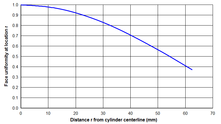
图 1 绘出了方程 \eqref{eq:11005a} 的曲线,对象为以 20 kHz 作轴向振动的 Ø125 mm Al 7075‑T6 圆柱体。
|
|
|
在 \( R \) 处(圆柱体外缘)对方程 \eqref{eq:11005a} 求值,即得到总体均匀性 \( \widehat{U} \)。
\begin{align} \label{eq:11006a} \widehat{U} = \frac{\textsf{Equation \eqref{eq:11001a} @ R}}{\textsf{Equation \eqref{eq:11004a}}} \end{align}
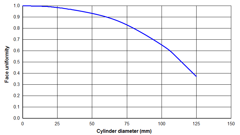
如果对不同直径的圆柱体计算方程 \eqref{eq:11006a},典型结果如图 2 所示。
|
|
|
注:可用来近似方程 \eqref{eq:11006a} 的更简单的三次方程,见附录 B。
径向振幅分布
对于半径为 \( R \) 的圆柱体,距圆柱体中心径向距离 \( r \) 处的径向振幅 \( U_{radial} \) 由下列方程给出。(见 Zemanek[1A],第 271 页,上方的方程 18。)
\begin{align} \label{eq:11007a} {U_{radial}}(r) = \Big[ \frac{h}{\gamma} \Big] \bigg\{ \Big[ 2 \, (\gamma \, R)^2 - \Omega^2 \Big] J_1(k \, R) \, J_1(h \, r) - \Big[ 2 \, (\gamma \, R)^2 \, J_1(h \, R) \, J_1(k \, r) \Big] \bigg\} \end{align}
在圆柱体外缘 \( r = R \) 处,上述方程变为 ——
\begin{align} \label{eq:11008a} {U_{radial}}(r=R) = \Big[ \frac{h}{\gamma} \Big] \bigg\{ \Big[ 2 \, (\gamma \, R)^2 - \Omega^2 \Big] J_1(k \, R) \, J_1(h \, R) - \Big[ 2 \, (\gamma \, R)^2 \, J_1(h \, R) \, J_1(k \, R) \Big] \bigg\} \end{align}
如果将方程 \eqref{eq:11008a} 除以方程 \eqref{eq:11004a},所得结果就是相对径向振幅(以轴向中心线振幅的百分比表示):
\begin{align} \label{eq:11009a} \widehat{U}_{radial} = \frac{\textsf{Equation \eqref{eq:11008a} @ R}}{\textsf{Equation \eqref{eq:11004a}}} \end{align}
结果表明,该方程的分子与分母符号相反。这表明当端面向外运动时波节处向内收缩,反之亦然。这正是泊松耦合所预期的现象。
(注:关于近似圆柱形变幅杆端面振幅分布的其他方程,见 Mori (1)。)
半波长变幅杆的最大适用直径
Pochhammer 方程是针对无限长圆柱体推导的。然而,圆柱形变幅杆的长度是有限的。事实证明,只要剪切应力远小于纵向应力,Pochhammer 方程对圆柱形变幅杆就是有效的。如果变幅杆直径相对于调谐半波长不是过大,这一条件就成立。Zemanek[1A](第 272 - 275 页)表明,只要 \( \Omega \) < 2.6,剪切应力就保持在纵向应力的 1% 以内(第 275 页)。(另见 Thurston,第 16 页。)将该值和 \( c_s \)(方程 \eqref{eq:11001a5})代入方程 \eqref{eq:11001a2} 并求解 \( D \)(即 \( 2R \)),得到:
\begin{align} \label{eq:11010a} D &\leq \Gamma_{tw} \, \left[ \frac{5.2}{\pi} \right] \, \left[ \frac{1}{2 \, (1 + \nu)} \right]^{1/2} \\[0.7em]%eqn_interline_spacing &\leq \left[ \frac{c_{tw}}{2 \, f} \right] \, \left[ \frac{5.2}{\pi} \right] \, \left[ \frac{1}{2 \, (1 + \nu)} \right]^{1/2} \nonumber \end{align}
其中 ——
| \( D \) | = 圆柱体直径 |
| \( f \) | = 频率 |
| \( c_{tw} \) | = 细丝波速 |
| \( \Gamma_{tw} \) | = 材料细丝半波长 |
| \( \nu \) | = 泊松比 |
采用 Al 7075‑T6 铝合金的材料常数(\( c_{tw} \) = 5081 m/sec,\( \nu \) = 0.33),上述方程表明,在 20 kHz 下 Pochhammer 方程对该铝材有效的最大直径约为 130 mm。超过 130 mm 后,Pochhammer 方程的误差将增大。事实上,Pochhammer 方程预测该铝制变幅杆在 150 mm 处会出现一个波节。这显然是不正确的,因为轴向谐振绝不应出现端面波节(除非受到邻近非轴向谐振的影响)。
除了直径限制之外,Pochhammer 方程还假设棒材是均质的。因此,它不考虑螺柱的影响。
附录 A — 贝塞尔函数
Pochhammer 方程中重要的贝塞尔函数具有以下特性(见 Kinsler,附录 A4,第 449 - 452 页)——
- J0(x),其中 \( x \) 为实数 —— \( J_0(x)\) 函数类似衰减的余弦函数,最大值为 1.0。
- \( J_0(jx) \),其中 \( jx \) 为虚数 —— \( J_0(jx)\) 函数取实数值,类似双曲余弦函数,其值随 \( x \) 增大而迅速增大。\( J_0(jx)\) 可表示为修正贝塞尔函数 \( I_0(x)\)(Kinsler,第 450 页)——
\begin{align} \label{eq:11035a} J_0(jx) = I_0(x) \end{align}
其中 \( I_0(x)\) 取实数值。 - J1(x),其中 \( x \) 为实数 —— \( J_1(x)\) 函数类似衰减的正弦函数,最大值约为 0.58。
- \( J_1(jx) \),其中 \( jx \) 为虚数 —— \( J_1(jx) \) 函数为虚数,类似双曲余弦函数,其值随 \( x \) 增大而迅速增大。\( J_1(jx) \) 可表示为修正贝塞尔函数(Kinsler,第 450 页)——
\begin{align} \label{eq:11036a} J_1(jx) = j I_1(x) \end{align}
其中 \( I_1(x)\) 取实数值。
对于高功率超声中关注的纵向谐振器,\( c_d \) 总是大于 \( c \)。因此,方程 \eqref{eq:11001a3} 中的 \( h \) 为虚数,因为方程 \eqref{eq:11001a3} 中 \( \sqrt{\textsf{ }} \) 根号下的值为负。于是,\( (h \, R) \) 和 \( J_1(h \, R) \) 均为虚数,它们在上述方程中的乘积因此是一个负实数。
附录 B — 多项式曲线拟合
虽然方程 \eqref{eq:11006a} 与实测均匀性吻合良好,但计算起来较为繁琐。因此,拟合了一个三次多项式方程 ——
\begin{align} \label{eq:11031a} \widehat{U} = 1 + b_2 \, \left( \frac{D}{\Gamma_{tw}} \right)^2 + b_3 \, \left( \frac{D}{\Gamma_{tw}} \right)^3 \end{align}
其中 ——
| \( \widehat{U} \) | = 指定圆柱体直径下的圆柱体均匀性 |
| \( D \) | = 圆柱体直径 |
| \( \Gamma_{tw} \) | = 细丝半波长 |
| \( b_2 \), \( b_3 \) | = 曲线拟合常数 |
注意,当圆柱体直径趋于零时,均匀性按要求趋于 1.0。此外,由于变幅杆直径为零时均匀性曲线的斜率应为零,因此该方程不含线性项 \( \left( D / \Gamma_{tw} \right)^1 \)(或者说,线性项的系数 \( b_1 \) 为 0)。
细丝半波长 \( \Gamma_{tw} \) 由下式计算 ——
\begin{align} \label{eq:11032a} \Gamma_{tw} = \frac{c_{tw}}{2 \, f} \end{align}
方程 \eqref{eq:11031a} 是在频率 20 kHz、波速 5081、泊松比 0.33(对应 Al 7075‑T6 铝合金)的条件下,针对 0 到 125 mm 之间的 7 个直径对 Pochhammer 方程进行拟合的。由此得到曲线拟合常数 ——
\begin{align} \label{eq:11033a} b_2 = -0.24744 \end{align}
\begin{align} \label{eq:11034a} b_3 = -0.40538 \end{align}
估计标准误差为 0.32。
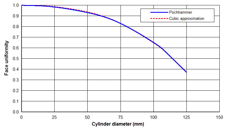
采用 \eqref{eq:11033a} 和 \eqref{eq:11034a} 中拟合常数的方程 \eqref{eq:11031a} 绘于图 B1 中。
|
|
|
如果材料属性与上述假设值相差较大,则计算出的均匀性将出现误差。幸运的是,大多数声学材料的材料属性都与铝相当接近,因此方程 \eqref{eq:11031a} 对这些材料应能给出合理的结果。
Pochhammer Amplitude Distributions
in an Infinitely Long Cylinder
Contents
In 1876, Pochhammer originally developed the equations for wave propogation in an infinitely long elastic cylinder with isotropic material properties. These equations predict the axial and radial amplitude distributions. (Note: the Pochhammer solution is sometimes called the Pochhammer-Chree solution or the Pochhammer-Love solution.)
The following has been taken essentially from Zemanek[1A]).
Axial amplitude distribution
For a cylinder of radius R, the axial amplitude \( U_{axial} \) at a radial distance \( r \) from the center of the cylinder is given by the following equation. (See Zemanek[1A], p. 271, lower equation 18.)
\begin{align} \label{eq:11001a} {U_{axial}}(r) = \Big[2 \, (\gamma \, R)^2 - \Omega^2 \Big] J_1(k \, R) \, J_0(h \, r) + \Big[ 2 \, (k \, R) \, (h \, R) \, J_1(h \, R) \, J_0(k \, r) \Big] \end{align}
where —
\begin{align} \label{eq:11001a1} \tag{1a} \gamma = \frac{2 \pi \, f}{c} \end{align}
\begin{align} \label{eq:11001a2} \tag{1b} \Omega = \frac{2 \pi \, f \, R}{c_s} \end{align}
\begin{align} \label{eq:11001a3} \tag{1c} h = 2 \pi \, f \, \left[ \frac{1}{{c_d}^2} - \frac{1}{{c}^2} \right]^{1/2} \end{align}
\begin{align} \label{eq:11001a4} \tag{1d} k = 2 \pi \, f \, \left[ \frac{1}{{c_s}^2} - \frac{1}{{c}^2} \right]^{1/2} \end{align}
\begin{align} \label{eq:11001a5} \tag{1e} c_s = c_{tw} \left[ \frac{1}{2 \, (1 + \nu)} \right]^{1/2} \end{align}
\begin{align} \label{eq:11001a6} \tag{1f} c_d = c_{tw} \left[ \frac{1 - \nu}{(1 + \nu) \, (1 - 2\nu)} \right]^{1/2} \end{align}
\begin{align} \label{eq:eq:11001a7} \tag{1g} c_{tw} = \left[ \frac{E}{\rho} \right]^{1/2} \end{align}
where —
| \( U_{axial}(r) \) | = axial amplitude at radius \( r \) |
| \( r \) | = radius at which the amplitude will be evaluated |
| \( R \) | = radius of cylinder |
| \( f \) | = frequency |
| \( c \) | = effective wave speed of the cylinder whose radius is \( R \) |
| \( c_{tw} \) | = thin-wire wave speed |
| \( c_s \) | = shear wave speed |
| \( c_d \) | = dilitational wave speed |
| \( \nu \) | = Poisson's ratio |
| \( J_0 \) | = Bessel function of the first kind, order 0 |
| \( J_1 \) | = Bessel function of the first kind, order 1 |
Each Bessel function operates on the parameter in ( ) (i.e., the Bessel function argument). (See Appendix A for further notes on Bessel functions.)
\( c_s \) and \( c_d \) can be evaluated from various material constants. (See the chapter on "Wave Motion".) However, unlike \( c_s \) and \( c_d \), \( c \) is not a material constant. Instead, \( c \) depends on the cylinder diameter. For the chosen cylinder diameter, \( c \) can be determined from the Pochhammer frequency equation. (See Zemanek[1A], p. 267, equation 6. Also see the chapter on "Wave Motion".) However, the solution of this equation is difficult. Instead, \( c \) can more easily be determined by the Mori equation. (See the chapter on "Wave Motion".)
Note that both \( c_s \) and \( c_d \) depend on Poisson's ratio \( \nu \). Hence, the axial amplitude distribution as well as the radial amplitude (below) will also depend on Poisson's ratio.
In the above equation, if \( r = 0 \) then \( U \) represents the axial amplitude at the axis of the cylinder. For \( r = 0 \) two of the Bessel functions evaluate to 1:
\begin{align} \label{eq:11002a} J_0(h \, r) = J_0(0) = 1 \end{align}
\begin{align} \label{eq:11003a} J_0(k \, r) = J_0(0) = 1 \end{align}
Then, the axial amplitude at the center of the cylinder is —
\begin{align} \label{eq:11004a} {U_{axial}}(r=0) = \Big[2 \, (\gamma \, R)^2 - \Omega^2 \Big] J_1(k \, R) + \Big[ 2 \, (k \, R) \, (h \, R) \, J_1(h \, R) \Big] \end{align}
If equation \eqref{eq:11001a} is evaluated at \( r \) and divided by equation \eqref{eq:11004a}, the result is \( \widehat{U}(r) \) (i.e., the uniformity at radius \( r \)):
\begin{align} \label{eq:11005a} \widehat{U}(r) = \frac{\textsf{Equation \eqref{eq:11001a} @ r}}{\textsf{Equation \eqref{eq:11004a}}} \end{align}
Equation \eqref{eq:11005a} is graphed in figure 1 for a Ø125 mm Al 7075‑T6 cylinder that vibrates axially at 20 kHz.
|
|
|
Evaluating equation \eqref{eq:11005a} at \( R \) (the cylinder periphery) gives the overall uniformity \( \widehat{U} \).
\begin{align} \label{eq:11006a} \widehat{U} = \frac{\textsf{Equation \eqref{eq:11001a} @ R}}{\textsf{Equation \eqref{eq:11004a}}} \end{align}
If equation \eqref{eq:11006a} is evaluated for cylinders of various diameters, a typical result is shown in figure 2.
|
|
|
Note: see Appendix B for a simpler cubic equation that approximates equation \eqref{eq:11006a}.
Radial amplitude distribution
For a cylinder of radius \( R \), the radial amplitude \( U_{radial} \) at a radial distance \( r \) from the center of the cylinder is given by the following equation. (See Zemanek[1A], p. 271, upper equation 18.)
\begin{align} \label{eq:11007a} {U_{radial}}(r) = \Big[ \frac{h}{\gamma} \Big] \bigg\{ \Big[ 2 \, (\gamma \, R)^2 - \Omega^2 \Big] J_1(k \, R) \, J_1(h \, r) - \Big[ 2 \, (\gamma \, R)^2 \, J_1(h \, R) \, J_1(k \, r) \Big] \bigg\} \end{align}
At the periphery of the cylinder \( r = R \) the above equation becomes —
\begin{align} \label{eq:11008a} {U_{radial}}(r=R) = \Big[ \frac{h}{\gamma} \Big] \bigg\{ \Big[ 2 \, (\gamma \, R)^2 - \Omega^2 \Big] J_1(k \, R) \, J_1(h \, R) - \Big[ 2 \, (\gamma \, R)^2 \, J_1(h \, R) \, J_1(k \, R) \Big] \bigg\} \end{align}
If equation \eqref{eq:11008a} is divided by equation \eqref{eq:11004a} then the result is the relative radial amplitude (as a percent of the axial centerline amplitude):
\begin{align} \label{eq:11009a} \widehat{U}_{radial} = \frac{\textsf{Equation \eqref{eq:11008a} @ R}}{\textsf{Equation \eqref{eq:11004a}}} \end{align}
It turns out that the numerator and denominator of this equation have opposite signs. This indicates that when the face is moving outward the node is collapsing inward and vice versa. This is expected from Poisson coupling.
(Note: See Mori (1) for other equations that approximate the face amplitude distribution in a cylindrical horn.)
Maximum applicable diameter for half-wave horns
The Pochhammer equation was developed for an infinitely long cylinder. However, cylindircal horns have finite length. It turns out that the Pochhammer equation is valid for cylindrical horns as long as the shear stresses are small compared to the longitudinal stresses. This will be true if the horn diameter is not excessively large compared to the tuned half-wavelength. Zemanek[1A] (pp. 272 - 275) shows that the shear stresses remain less than 1% of the longitudinal stress as long as \( \Omega \) < 2.6 (p. 275)). (Also see Thurston, p. 16.) Substituting this value and \( c_s \) (equation \eqref{eq:11001a5}) into equation \eqref{eq:11001a2} and solving for \( D \) (i.e., \( 2R \)) gives:
\begin{align} \label{eq:11010a} D &\leq \Gamma_{tw} \, \left[ \frac{5.2}{\pi} \right] \, \left[ \frac{1}{2 \, (1 + \nu)} \right]^{1/2} \\[0.7em]%eqn_interline_spacing &\leq \left[ \frac{c_{tw}}{2 \, f} \right] \, \left[ \frac{5.2}{\pi} \right] \, \left[ \frac{1}{2 \, (1 + \nu)} \right]^{1/2} \nonumber \end{align}
where —
| \( D \) | = diameter of cylinder |
| \( f \) | = frequency |
| \( c_{tw} \) | = thin-wire wave speed |
| \( \Gamma_{tw} \) | = material thin-wire half-wavelength |
| \( \nu \) | = Poisson's ratio |
Using the material constants for Al 7075‑T6 aluminum ( \( c_{tw} \) = 5081 m/sec, \( \nu \) = 0.33), the above equation indicates that the maximum diameter for which the Pochhammer equation is valid for this aluminum at 20 kHz is approximately 130 mm. Above 130 mm, the Pochhammer equation will have increased error. In fact, the Pochhammer equation predicts that the aluminum horn will a node at 150 mm. This is obviously incorrect, since an axial resonance should never have a face node (except when influenced by an adjacent nonaxial resonance).
In addition to the limiting diameter, the Pochhammer equation also assumes that the rod material is homogeneous. Therefore, it does consider the effect of a stud.
Appendix A — Bessel Functions
The important Bessel functions for the Pochhammer equation have the following characteristics (see Kinsler, appendix A4, pp. 449 - 452) —
- J0(x), where \( x \) is a real number — The \( J_0(x)\) function resembles a decaying cosine function and has a maximum value of 1.0.
- \( J_0(jx) \), where \( jx \) is an imaginary number — The \( J_0(jx)\) function is real valued and resembles a hyperbolic cosine function, whose value rapidly increases as \( x \) increases. \( J_0(jx)\) can be expressed as a modified Bessel function \( I_0(x)\) (Kinsler, p. 450) —
\begin{align} \label{eq:11035a} J_0(jx) = I_0(x) \end{align}
where \( I_0(x)\) is real valued. - J1(x), where \( x \) is a real number — The \( J_1(x)\) function resembles a decaying sine function and has a maximum value of about 0.58.
- \( J_1(jx) \), where \( jx \) is an imaginary number — The \( J_1(jx) \) function is imaginary and resembles a hyperbolic cosine function, whose value rapidly increases as \( x \) increases. \( J_1(jx) \) can be expressed as a modified Bessel function (Kinsler, p. 450) —
\begin{align} \label{eq:11036a} J_1(jx) = j I_1(x) \end{align}
where \( I_1(x)\) is real valued.
For longitudinal resonators that are of interest in high-power ultrasonics, \( c_d \) is always greater than \( c \). Thus, \( h \) from equation \eqref{eq:11001a3} is imaginary since the value under the \( \sqrt{\textsf{ }} \) in equation \eqref{eq:11001a3} is negative. Thus, \( (h \, R) \) and \( J_1(h \, R) \) are both imaginary and their product in the above equations is thus a negative real number.
Appendix B — Polynomial Curve-fit
While equation \eqref{eq:11006a} agrees well with measured uniformities, it can be cumbersome to calculate. Therefore, a cubic polynomial equation has been fitted —
\begin{align} \label{eq:11031a} \widehat{U} = 1 + b_2 \, \left( \frac{D}{\Gamma_{tw}} \right)^2 + b_3 \, \left( \frac{D}{\Gamma_{tw}} \right)^3 \end{align}
where —
| \( \widehat{U} \) | = cylinder uniformity for specified cylinder diameter |
| \( D \) | = cylinder diameter |
| \( \Gamma_{tw} \) | = thin-wire half-wavelength |
| \( b_2 \), \( b_3 \) | = curve fit constants |
Note that as the cylinder diameter goes to zero the uniformity goes to 1.0, as required. Also, since the slope of the uniformity curve should be zero when the horn diameter is zero, the equation has no linear term \( \left( D / \Gamma_{tw} \right)^1 \) (or, alternately, the coefficient \( b_1 \) of the linear term is 0).
The thin-wire half-wavelength \( \Gamma_{tw} \) is calculated from the equation —
\begin{align} \label{eq:11032a} \Gamma_{tw} = \frac{c_{tw}}{2 \, f} \end{align}
Equation \eqref{eq:11031a} was fitted to the Pochhammer equation for 7 diameters ranging between 0 and 125 mm at a frequency of 20 kHz with a wave speed of 5081 and Poisson's ratio of 0.33 (corresponding to Al 7075‑T6 aluminum). This yielded the curve-fit constants —
\begin{align} \label{eq:11033a} b_2 = -0.24744 \end{align}
\begin{align} \label{eq:11034a} b_3 = -0.40538 \end{align}
with a the standard error of estimate 0.32.
Equation \eqref{eq:11031a} with the fit constants from \eqref{eq:11033a} and \eqref{eq:11034a} is graphed in figure B1.
|
|
|
If the material properties vary significantly from the above assumed values then the calculated uniformity will err. Fortunately, most acoustic materials have material properties that are reasonably close to aluminum so equation \eqref{eq:11031a} should give reasonable results for these materials.