附录 G:理解压电参数
本附录介绍各种压电参数与常数之间的关系,以及机械和电学边界条件对这些参数的影响。
注 —
- 以下讨论使用压电文献中常见的符号。这些符号与弹性力学中传统使用的符号不同。
- 下面的公式通常用单个符号来表示陶瓷的某一特性。然而实际上,该符号往往代表一个属性常数矩阵。例如,弹性柔度用 \( s \) 表示,它实际上是矩阵 —
- 下面的公式假设为线性行为,这在低驱动电平下成立。然而,陶瓷在高驱动电平下会呈现非线性行为;尽管如此,这些公式仍可为各参数之间的关系提供指导。
|
||||||||||||
|
\begin{align} \label{eq:10001b} \nonumber s = \left[ \begin{matrix} s_ {11} &s_ {12} &s_ {13} &0 &0 &0 \\ s_ {21} &s_ {22} &s_ {23} &0 &0 &0 \\ s_ {31} &s_ {32} &s_ {33} &0 &0 &0 \\ 0 &0 &0 &s_ {44} &0 &0 \\ 0 &0 &0 &0 &s_ {55} &0 \\ 0 &0 &0 &0 &0 &s_ {66} \\ \end{matrix} \right] \end{align}
为避免处理此类矩阵带来的复杂性,且不失一般性,以下假设所有应力均为单轴应力(即不存在横向应力或剪切应力),并假设压电材料为各向同性。(事实上,压电陶瓷可能具有很强的各向异性。例如,Piezo Technologies(第 6 页)指出:"径向声速通常比轴向声速高 20% 到 30%。")
基本压电关系
所有固体在受到外力作用时都会发生变形。应变 \( S \) 与应力 \( T \) 之间的关系为 —
\begin{align} \label{eq:10001a} S &= s \,T \end{align}
式中 \( s \)(小写)为材料的柔度(杨氏模量的倒数)。该公式假设 \( S \) 与 \( T \) 之间为线性关系,至少在所关注的范围内如此。后续所有公式都将假设这种线性关系。
如果材料是电介质(如电容器),则面电荷密度 \( D \) 与所加电场 \( E \) 之间的关系为 —
\begin{align} \label{eq:10002a} D &= \varepsilon \,E \end{align}
式中 \( \varepsilon \) 为材料的介电常数。上述参数汇总于表 G2。
|
|||||||||||||||||||||
|
注意,公式 \eqref{eq:10001a} 和 \eqref{eq:10002a} 不涉及任何压电效应(即公式 \eqref{eq:10001a} 的机械效应与公式 \eqref{eq:10002a} 的电学效应之间没有相互作用)。然而,如果材料具有压电性,则必须在每个公式中添加一个附加项来表征压电效应。对于逆压电效应(电场使材料产生应变),必须在公式 \eqref{eq:10001a} 中添加 \( d^T E \) 项。
\begin{align} \label{eq:10003a} S &= s^E \,T + d^T \,E \end{align}
式中 \( d \) 为压电电荷常数(见表 G4)(表示约束的上标将在下文解释)。加入电荷常数 \( d^T \) 后,即使应力 \( T \) 为零,应变 \( S \) 也可以不为零(由电场 \( E \) 引起)。
另一种与之互补的压电效应是:外部应力使压电材料中积累电荷。(这就是正压电效应,最早由居里夫妇研究。)为表征该效应,必须在公式 \eqref{eq:10002a} 中添加 \( d^E T \) 项。
\begin{align} \label{eq:10004a} D &= \varepsilon^T \,E + d^E \,T \end{align}
式中 \( d \) 同样是压电电荷常数。加入电荷常数 \( d^E \) 后,即使电场 \( E \) 为零,电荷 \( D \) 也可以不为零(由应力 \( T \) 引起)。
注意,如果 \( d \) = 0(即材料不具有压电性),则公式 \eqref{eq:10003a} 和 \eqref{eq:10004a} 就分别退化为公式 \eqref{eq:10001a} 和 \eqref{eq:10002a}。因此,材料的压电特性由电荷常数项 \( d^T \) 和 \( d^E \) 定义。
公式注 —
- 公式 \eqref{eq:10003a} 和 \eqref{eq:10004a} 实际上并不完整,因为其他参数也可能影响性能。例如,材料温度变化时应变 \( S \) 也会改变。因此,应添加 \( \alpha H \) 之类的项,其中 \( \alpha \) 为热膨胀系数,\( H \) 为温升。
\begin{align} \label{eq:10099a} S &= s^E \, T + d^T \, E + α \, H \end{align}
因此,温度对应变的影响方式与电场类似。如果材料是磁致伸缩材料,则还应考虑磁致伸缩效应。此处给出的公式隐含地假设这些效应不存在(例如,材料保持恒温)或可以忽略。 - 虽然公式 \eqref{eq:10003a} 和 \eqref{eq:10004a} 通常以当前形式给出,但可以很容易地重新排列变量,得到其他形式的公式。
上标(约束边界条件)
常数上的上标表示该上标参数保持恒定(受约束)。例如,考虑公式 \eqref{eq:10003a} 中带上标 \( E \) 的柔度参数 \( s \)(即 \( s^E \))。\( s^E \) 表示在测定弹性柔度 \( s \) 时(例如对材料进行应力-应变拉伸试验时),电场强度 \( E \) 保持恒定。如果 \( E \) 不保持恒定,则应变 \( S \) 中有一部分将来自 \( d^T E \) 的压电效应,\( S \) 的测量值就不正确。(同样,在应力-应变拉伸试验中保持温度恒定,使应变只受应力影响,而不受热膨胀影响。)
同样,公式 \eqref{eq:10004a} 中的介电常数 \( \varepsilon \) 只有在应力 \( T \) 保持恒定时才能正确测定(即 \( \varepsilon^T \))。否则,电位移 \( D \) 中有一部分将由应力 \( T \) 而非电场 \( E \) 引起,\( \varepsilon \) 的测量值就不正确。
常见约束汇总于表 G3。
|
|||||||||||||||
|
表 G3 注 —
- 通过物理约束压电陶瓷无法实际实现恒定应变状态。然而,可以在非常高的频率下激励来实现 —— 此时惯性效应大到陶瓷实际上无法振动(即不存在应变)。(见 Cady (1),第 328、572 页。)当单自由度弹簧-质量系统在远高于其谐振频率的频率下受激励时,也会出现同样的情况 —— 质量块将保持在静止位置不动。
- 恒定电场(恒定 \( E \))条件最容易通过将陶瓷的电极面短路来实现,使电场无法存在(即 \( E=0 \))。因此,在恒定电场 \( E \) 下测定的参数可称为短路参数。
- 恒定电位移(恒定 \( D \))条件最容易通过将陶瓷的电极面开路来实现,使电流无法流通(即 \( D=0 \))。因此,在恒定电位移 \( D \) 下测定的参数可称为开路参数。
基于上述约束,表 G4 列出了几个压电陶瓷参数。这些参数之间的关系将在后面讨论。
|
|||||||||||||||||||||
|
电荷常数 \( d \) 的意义
当换能器用作发射器时(如本站所述的应用),电荷常数 \( d^T \) 尤为重要,因为它决定了施加电场时压电材料膨胀或收缩的程度(称为逆压电效应)。在这种情况下,希望电荷常数较大,以便在给定电场下获得较大的振幅(位移)。
(当换能器用作接收器时,\( d^E \) 决定压电材料受应力作用时产生的电荷量(称为正压电效应)。然而,对于功率换能器,正压电效应相对不重要,除非换能器中使用单独的压电陶瓷作为电反馈来监测换能器的振幅。)
尽管 \( d^T \) 和 \( d^E \) 的单位不同,但它们在国际单位制(S.I.)中的数值相同(见 Berlincourt (3),公式 24a,第 188 页)。因此,公式 \eqref{eq:10003a} 和 \eqref{eq:10004a} 通常省略 \( d \) 上的 \( T \) 和 \( E \) 上标。
\begin{align} \label{eq:10007a} S &= s^E \,T + d \,E \end{align}
\begin{align} \label{eq:10008a} D &= \varepsilon^T \,E + d \,T \end{align}
公式的其他形式
如上所述,这些公式可以重新排列以得到其他常数。例如,从公式 \eqref{eq:10008a} 解出 \( E \) 并代入公式 \eqref{eq:10007a},可得 —
\begin{align} \label{eq:10009a} S &=s^{E} \,T + \frac{d}{\varepsilon^{T}}D - \frac{d^{2}}{\varepsilon^{T}} T \\[0.7em]%complex_eqn_interline_spacing &= s^{E} \,T + \frac{d}{\varepsilon^{T}}D - \frac{s^{E}}{s^{E}} \frac{d^{2}}{\varepsilon^{T}} T \nonumber \\[0.7em]%complex_eqn_interline_spacing &= s^{E}\left[1 - \frac{d^{2}}{s^{E} \varepsilon^{T}}\right] T + \frac{d}{\varepsilon^{T}} D \nonumber \end{align}
将常数因子合并为两个新常数,公式 \eqref{eq:10009a} 可简化 — 即
\begin{align} \label{eq:10010a} \kappa &=\frac{d}{\left(s^{E} \varepsilon^{T}\right)^{1/2} } \end{align}
\begin{align} \label{eq:10011a} g^{T} =\frac{d}{\varepsilon ^{T}} \end{align}
式中 —
|
|||||||||
|
(\( \kappa \) 的另一种推导及其意义的说明见压电耦合系数一节。)
于是 \eqref{eq:10009a} 变为 —
\begin{align} \label{eq:10012a} S=s^{E} (1 - \kappa^{2}) \,T + g^{T} D \end{align}
如果 \( D \) 保持恒定(例如,断开电极(开路)使电荷无法流动 — 即 \( D \) = 0),则公式 \eqref{eq:10012a} 变为 —
\begin{align} \label{eq:10013a} S=\left[s^{E} (1 - \kappa^{2})\right] \,T \end{align}
公式 \eqref{eq:10013a} 定义了陶瓷电极开路(即 \( D \) = 恒定)时应变与应力之间的关系。因此,因子 \( s^E (1 - \kappa^2) \) 就是开路柔度,记为 \( s^D \) —
\begin{align} \label{eq:10014a} s^{D} = s^E(1 - \kappa^{2}) \end{align}
然后将公式 \eqref{eq:10014a} 代入公式 \eqref{eq:10012a},得 —
\begin{align} \label{eq:10015a} S=s^{D} \,T + g^{T} D \end{align}
(见 Berlincourt (3),公式 21a,第 188 页。)
与公式 \eqref{eq:10003a} 相比,公式 \eqref{eq:10015a} 中的应变 \( S \) 现在分别以应力 \( T \) 和电位移 \( D \) 表示,相应的常数为 \( s^D \) 和 \( g^T \)。公式 \eqref{eq:10003a} 与公式 \eqref{eq:10015a} 之间的选择完全是任意的(尽管公式 \eqref{eq:10003a} 更常用)。
杨氏模量
公式 \eqref{eq:10014a} 表明,压电陶瓷可以具有两种不同的柔度 \( s^E \) 和 \( s^D \)。这源于压电陶瓷机械特性与电学特性的耦合。
公式 \eqref{eq:10014a} 以柔度表示。然而,由于杨氏模量 \( Y \) 就是柔度 \( s \) 的倒数(即对于各向同性材料,\( Y=s^{-1} \) 或 \( Y=1/s \)),公式 \eqref{eq:10014a} 可写成 —
\begin{align} \label{eq:10016b} \frac{1}{Y^D} = \frac{1}{Y^E}(1 - \kappa^{2}) \end{align}
或
\begin{align} \label{eq:10016a} Y^D=\frac{Y^E}{1 - \kappa^{2}} \end{align}
式中 —
| \( Y^D \) | = 开路时的杨氏模量 |
| \( Y^E \) | = 短路时的杨氏模量 |
(如前所述,杨氏模量通常用 \( E \) 表示。然而,由于此处 \( E \) 用于表示电场强度,杨氏模量改用 \( Y \) 表示。)
因此,压电陶瓷具有两种不同的杨氏模量,取决于电学边界条件(短路或开路)。由于 \( \kappa \) 总是小于 1.0,开路模量 \( Y^D \) 总是大于短路模量 \( Y^E \)。
物理解释
本节对两种杨氏模量给出物理解释。(注 — 以下图形仅供示意。X 轴和 Y 轴网格没有特定比例,各图之间不能直接比较。)
考虑一块压电陶瓷,逐渐施加力直至 \( F \) 使其受压(见图 G1)。如果压电陶瓷的电极开路(无导电通路),则压缩能量的一部分用于建立电场(即由于压电陶瓷的电容而产生电荷分离);其余(被消耗的)能量用于使压电陶瓷变形。因此,力 \( F \) 产生位移 \( U_1 \). 这就是图中的实线。
现在,如果将受压的压电陶瓷短路,电场就会消失。电场的相关能量也随之消失,但由于这是一个保守系统,损失的电能必须转化为另一种形式的能量。转化的能量使压电陶瓷产生附加应变,位移从 \( U_1 \) 增加到 \( U_2\)(点划线)。因此,压电陶瓷在短路时的压缩量大于开路时。(如果压电陶瓷一开始就处于短路状态,则力 \( F \) 会直接将其变形至 \( U_2\)(虚线),而不经过中间的开路步骤。)
|
|
|
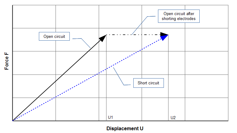
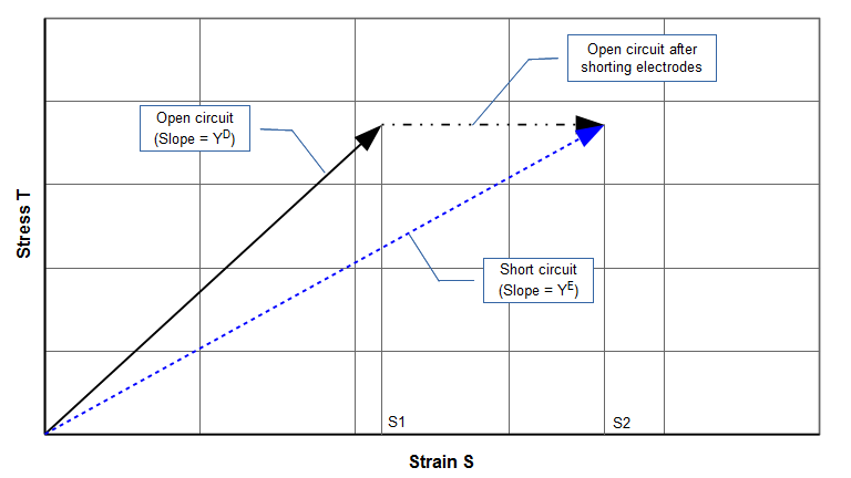
图 G1 可以转换为图 G2 中常见的应力-应变图。杨氏模量 \( Y \) 是相应应力-应变曲线的斜率。图 G2 表明,短路(虚)线的斜率低于开路(实)线(即对于给定应力,短路时的应变 \( S_2 \) 大于开路时的应变 \( S_1 \))。因此,短路时的杨氏模量(\( Y^E \))必然低于开路时的杨氏模量(\( Y^D \))。
|
|
|
压缩气体类比
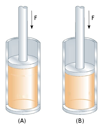
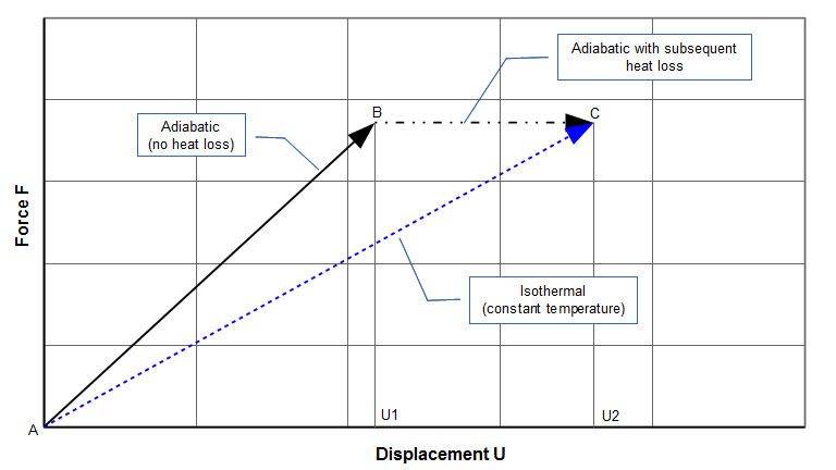
图 G3 所示为一个气缸,通过逐渐施加力直至 \( F \) 来压缩气体。左图中气缸是绝热的,热量无法逸出。这就是绝热条件(图 G4 中的实线 AB)。在压缩过程中,与未压缩状态相比,气体的温度(热能)升高了。热能的增加将位移限制为 \( U_1 \)。
现在假设多余的热能通过气缸壁散出,使温度恢复到原始状态。由于活塞力不变,热能的损失意味着气体在先前位置无法再支撑相同的活塞力;因此活塞下降到新的平衡位置 \( U_2 \) (右图气缸)。这就是图 G4 中的点划线 BC。
如果气缸在整个加载过程中不绝热,也会达到相同的终态 C。这样就不会有热能积累,加载将从 A 平稳地进行到 C(虚线)。这就是等温(恒温)条件。
因此,气体在等温条件(AC 线)下的压缩量大于绝热条件(AB 线),所以等温体积模量(\( B_T \))必然低于绝热体积模量(\( B_S \))。这与压电模量(\( Y \))类似 —— 短路模量(\( Y^E \))低于开路模量(\( Y^D \))。
|
|
|
|
|
|
短路谐振与开路谐振
由于压电陶瓷具有两种杨氏模量,它必然也有两个相关的谐振。与 \( Y^E \) 相关的谐振称为短路谐振 \( f_{sc} \)。与 \( Y^D \) 相关的谐振称为开路谐振 \( f_{oc} \)。(短路谐振也称为串联谐振;开路谐振也称为并联谐振。原因将在别处讨论。zzz explain distinction)这些谐振之间的关系如下所示。
由于谐振频率与杨氏模量的平方根成正比(即 \( f\propto \sqrt{Y} \)),公式 \eqref{eq:10016a} 可用短路谐振 \( f_{sc} \) 和开路谐振 \( f_{oc} \) 写成:
\begin{align} \label{eq:10018a} {f_{oc}}^2={f_{sc}}^2 \left(\frac{1}{1 - \kappa^{2}} \right) \end{align}
或
\begin{align} \label{eq:10019a} {f_{oc}}={f_{sc}} \, \sqrt{\frac{1}{1 - \kappa^{2}} } \end{align}
式中 —
| \( f_{sc} \) | = 短路谐振 |
| \( f_{oc} \) | = 开路谐振 |
注意,\( \kappa \) 的值介于 0 和 1 之间(见下文),因此公式 \eqref{eq:10019a} 根号下的量总是 \( \geq 1 \)。这意味着开路谐振 \( f_{oc} \) 总是大于短路谐振 \( f_{sc} \);相对差值取决于耦合系数 \( \kappa \)。
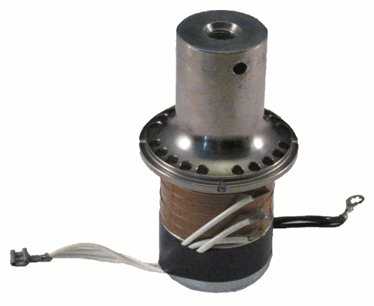
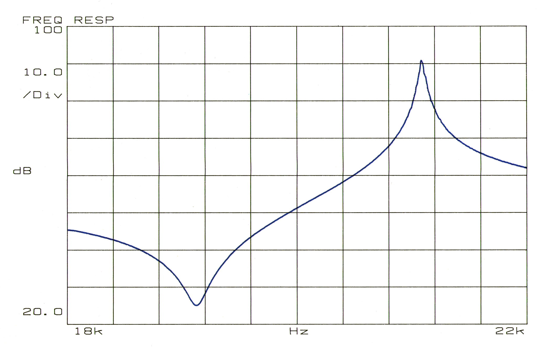
图 G6 所示为图 G5 中 20 kHz 换能器(Branson 502)的频率响应阻抗图。阻抗谷值对应短路谐振 \( f_{sc} \),阻抗峰值对应开路谐振 \( f_{oc} \)。(该换能器设计为在开路(并联)谐振下工作。开路谐振频率(约 20.8 kHz)略高于 20 kHz 的设计频率,因为该换能器没有前螺柱。加装前螺柱会使频率降至所需的工作范围。)
|
|
|
|
|
|
压电耦合系数 κ — 物理含义
储存在压电材料中的能量可以有三种形式 — 弹性(应变)能、电容电能和耦合机电能。为说明这一点,将公式 \eqref{eq:10007a} 和 \eqref{eq:10008a} 用能量表示 —— 将 \eqref{eq:10007a} 各项乘以 \( T \)/2、\eqref{eq:10008a} 各项乘以 \( E \)/2:
\begin{align} \label{eq:10020a} \small\frac{1}{2}\normalsize \,S \,T &= \small\frac{1}{2}\normalsize \,s^E \,T^2 + \small\frac{1}{2}\normalsize \,d \,E \,T \end{align}
\begin{align} \label{eq:10021a} \small\frac{1}{2}\normalsize \,D \,E &= \small\frac{1}{2}\normalsize \,\varepsilon^T \,E^2 + \small\frac{1}{2}\normalsize \,d \,E \,T \end{align}
注意,这些公式中的能量实际上是能量密度(即单位体积的能量)。
在公式 \eqref{eq:10020a} 中,\( \frac{1}{2} S \, T \) 为储存的总机械能,由应变能 \( \widehat{W}_1 \)(\( = \frac{1}{2} s^E \, T^2\))和耦合压电能 \( \widehat{W}_{12} \)(\( = \frac{1}{2} d \,E \, T \))组成。
在公式 \eqref{eq:10021a} 中,\( \frac{1}{2} D \, E \) 为储存的总电能,由储存的电容能 \( \widehat{W}_2 \)(\( = \frac{1}{2} \varepsilon^T \, E^2\))以及同样出现的耦合压电能 \( \widehat{W}_{12} \)(\( = \frac{1}{2} d \,E \, T \))组成。
耦合系数 \( \kappa \) 可用上述能量表示为(Waanders (1),公式 A8,第 84 页;或 Berlincourt (3),公式 30,第 190 页) —
\begin{align} \label{eq:10022a} \kappa &= \frac{\widehat{W}_{12}}{(\widehat{W}_1 \,\widehat{W}_2)^{1/2}} \end{align}
式中 —
| \( \kappa \) | = 压电耦合系数 |
| \( \widehat{W}_1 \) | = 储存的总机械能 |
| \( \widehat{W}_2 \) | = 储存的总电能 |
| \( \widehat{W}_{12} \) | = 耦合压电能 |
因此,耦合系数是耦合压电能与储存机械能和储存电能的几何平均值之比。
将公式 \eqref{eq:10020a} 和 \eqref{eq:10021a} 中的具体能量项代入 \eqref{eq:10022a},得 —
\begin{align} \label{eq:10023a} \kappa &= \frac{\frac{1}{2} \,d \,E \,T}{\left[(\frac{1}{2} \,s^E \,T^2) \,(\frac{1}{2} \,\varepsilon^T \,E^2)\right] ^{1/2}} \\[0.7em]%complex_eqn_interline_spacing &=\frac{d}{\left(s^{E} \, \varepsilon^{T}\right)^{1/2} } \nonumber \end{align}
注意,从能量角度推导出的公式 \eqref{eq:10023a} 与公式 \eqref{eq:10010a} 相同。
对于单片压电陶瓷,\( \kappa \) 取决于元件的形状、激励模式(例如纵向、径向、厚度方向)和边界条件。表 G6 列出了评估单片压电陶瓷 \( \kappa \) 时最常见的条件。\( \kappa \) 的下标表示规定的条件(符号约定见此处)。
|
||||||||||||||||||||||||||||||
|
上述定义的耦合系数可用于规定或评估单片压电陶瓷的性能,也可用作与完整装配的换能器进行比较的参考值。
用于确定耦合系数的公式 \eqref{eq:10019a} 既可用于任意条件(任意形状、约束等)下的单片压电陶瓷,也可用于整个换能器。对于后一种情况,相应术语就成为有效压电耦合系数 \( \kappa_{eff} \)。(或者,\( \kappa_{33} \)、\( \kappa_{31} \)、\( \kappa_{t} \)、\( \kappa_{p} \) 和 \( \kappa_{u} \) 可以视为更一般的 \( \kappa_{eff} \) 的特例。)Woollett (1)(第 24 页)指出:"然而,换能器的耦合系数通常低于其制造所用材料的耦合系数,因此称为有效 \( \kappa \),以区别于材料的 \( \kappa \)。"\( \kappa \) 的有效值(即 \( \kappa_{eff} \))取决于具体换能器的设计(例如叠堆螺栓的影响、陶瓷的布置和长度等)。
注意,大多数功率换能器以 33 模式振动。然而,\( \kappa_{33} \) 并不适用于这种模式,因为它针对的是细长棒或杆。应改用 \( \kappa_{t} \),因为它针对的是薄圆片。
由公式 \eqref{eq:10018a} 或 \eqref{eq:10019a},任何耦合系数都可以由其相关的开路谐振 \( f_{oc} \) 和短路谐振 \( f_{sc} \) 频率计算得出。(另见 Waanders (1),公式 A19a,第 85 页。)
\begin{align} \label{eq:10024a} \kappa _{eff} &= \left[1 - \left( \frac{ f_{sc} } { f_{oc} } \right)^2 \right]^{1/2} \end{align}
所需频率可以通过解析分析或实测实际压电陶瓷或装配好的换能器获得。例如,对于图 G5 中的换能器,开路频率和短路频率(从图 G6 得到)分别为 20.8 kHz 和 18.8 kHz。因此,该换能器的 \( \kappa_{eff} \) 为 0.43。
κ 的意义
Berlincourt (3)(第 189 页)断言:"压电材料最重要的性质是其压电耦合系数。"
\( \kappa \) 的意义可由公式 \eqref{eq:10022a} 确定。分子代表转换的能量,分母代表总输入能量(Waanders (1),第 12 页)。
\begin{align} \label{eq:10025a} \kappa &= {\left[\frac{\text{Energy converted}}{\text{Energy input}} \right]}^{1/2}_{\text {Low frequency}} \end{align}
由于"转换的能量"必须总是小于"输入的能量",\( \kappa \) 必须总是小于 1.0。
为获得最大的压电效应,应尽可能多地将输入能量转换为压电能。因此,单片陶瓷的 \( \kappa \) 和装配好的换能器的 \( \kappa_{eff} \) 都应尽可能大。最大化 \( \kappa \) 同时也会使 \( d \) 和功率最大化。
最大化的 \( d \)
见公式 \eqref{eq:10023a}。这将使输出振幅最大化。
最大化的功率
Berlincourt (3)(第 250 页,公式 147)给出了超声换能器可产生的理论功率公式。
\begin{align} \label{eq:10026a} p &= 2 \pi f_{sc} \, {E_3}^2 \, \kappa^2 \, \varepsilon_{33}^T \, Q_M \end{align}
式中 —
| \( p \) | = 声功率密度(单位体积压电陶瓷的功率)[W/m3] |
| \( f_{sc} \) | = 短路(串联)谐振频率 [Hz] |
| \( E_3 \) | = 电场强度 [VRMS/m] |
| \( \kappa \) | = 机电耦合系数 [无单位] |
| \( \varepsilon_{33}^T \) | = 恒定应力下的压电介电常数 [(coulomb/volt)/m = Farad/m] |
| \( Q_M \) | = 机械品质因数 Q [无单位] |
注意,该公式本身并未对参数(尤其是电场强度 \( E \))施加任何限制。实际上,必须限制 \( E \),以防止损坏压电陶瓷(取决于压电陶瓷的类型)、防止损耗不必要地增加,以及防止压电陶瓷表面之间或对其他表面发生电弧放电。
为获得可输出的实际功率 \( P \),公式 \eqref{eq:10026a} 各项必须乘以压电陶瓷体积 \( \widetilde{V} \) [m3]。
\begin{align} \label{eq:10027a} P &= 2 \pi f_{sc} \, {E_3}^2 \, \tilde{V} \, \kappa^2 \, \varepsilon_{33}^T \, Q_M \end{align}
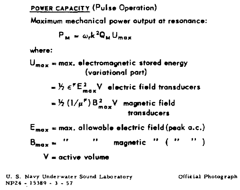
公式 \eqref{eq:10027a} 与 Woollett (1)(第 26 页)的公式等价(见此处图 G7)。Wollett(第 24 页)指出,他的公式是"在发热和弹性失效不是控制因素时,对脉冲应用中换能器功率容量的粗略估计"。具体的工作制无法确定,因为它取决于冷却、热传导等因素。(注意,Wollett 的公式规定 \( E_{max} \) 为"交流峰值"。因此,Wollett 的公式中有一个 ½ 因子,用于将 \( E_{max}^2 \) 转换为有效值。)
|
|
|
因此,公式 \eqref{eq:10026a} 和 \eqref{eq:10027a} 表明,声功率与机电耦合系数的平方成正比。
Berlincourt 的公式基于两个假设 ——
- 假设 —— 换能器可表示为集总参数系统(例如 Berlincourt 的陶瓷居中的大质量负载换能器)。事实上,实际换能器并不符合这一理想模型,因为明显的应变会延伸到两端质量块中。在这种情况下,\( \kappa \) 应替换为 \( \kappa_{eff} \).(见 Woollett (1),第 24 页 —— "然而,换能器的耦合系数通常低于其制造所用材料的耦合系数,因此称为有效 \( k \),以区别于[压电]材料的 \( k \)。")
- 假设 —— 换能器对控制参数(例如电场强度 \( E \))的响应是线性的。然而,在高驱动电平下,这一假设很可能不成立(Woollett (1),第 24 页)。例如,见下面来自 Berlincourt (2) 的图。当陶瓷在较高温度下工作时(通常由于内部发热),线性假设会被进一步破坏。
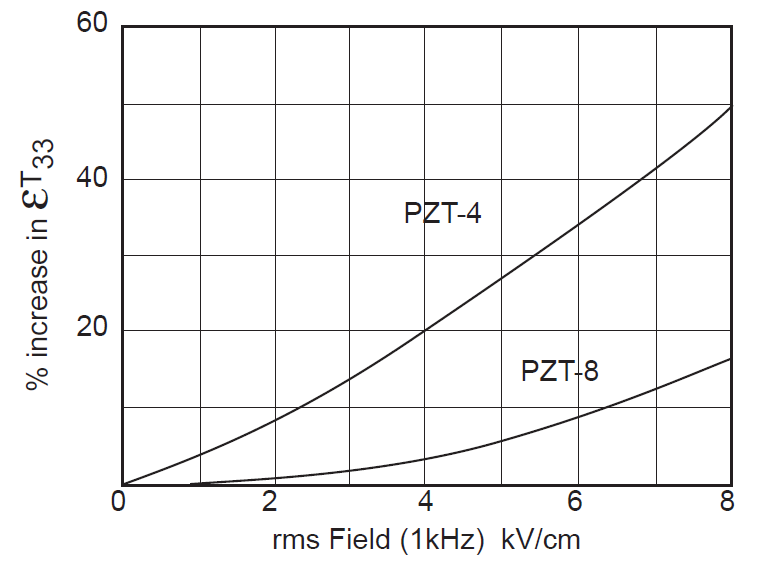
图 G8. 电场强度对压电陶瓷介电常数的影响
因此,Woollett (1)(第 24 页)指出,对于实际换能器,预测的功率将"相当近似"。然而,由于忽略了劣化因素(例如热因素),上述公式预测的功率或许应视为上限。
用于质量控制
有效机电耦合系数可用于对单片陶瓷进行部分合格鉴定 — 任何超出可接受范围的压电陶瓷都予以剔除。(\( \kappa_{eff} \) 通常应由压电陶瓷制造商提供。但请注意,制造商可能只是将其称为机电耦合系数或 \( \kappa \),而省略"有效"二字。)
同样,\( \kappa_{eff} \) 可用于鉴定整个换能器。如果某换能器的 \( f_{oc} \) 异常接近 \( f_{sc} \),使得 \( \kappa_{eff} \) 异常小(公式 \eqref{eq:10024a}),则很可能表明该换能器存在缺陷。(在这种情况下,将所选换能器的 \( \kappa_{eff} \) 与已知"良好"的、标称设计相同的换能器的平均 \( \kappa_{eff} \) 进行比较。)
不当使用
尽管 \( \kappa \) 很重要,但它有时会被误解。
比较换能器设计
不能基于 \( \kappa_{eff} \) 来比较不同的换能器设计。
考虑对换能器进行修改、使其储能增加的情况(例如,提高前质量块或后质量块的密度,或在前质量块上加工出增益结构)。此时 \( f_{oc} \) 与 \( f_{sc} \) 之间的差值会减小(从而降低 \( \kappa_{eff} \)),尽管功率承载能力并未受到影响。
因此,必须谨慎解读 \( \kappa_{eff} \)。正如 Waanders(第 82 页)所指出的:"根据[换能器的]结构不同,会得到不同的 \( \kappa_{eff} \) 值。要将其换算为绝对质量水平往往非常复杂,甚至不可能。"
还要注意,\( \kappa_{eff} \) 并未考虑任何换能器损耗。因此,两个换能器可能具有相同的 \( \kappa_{eff} \),但损耗却相差悬殊。
鉴于上述考虑,\( \kappa_{eff} \) 在比较不同设计的换能器时作用有限。
判断换能器损耗
由于并联和串联谐振频率基本上与换能器的机械损耗和电损耗无关(假设这些损耗在合理范围内),\( \kappa_{eff} \) 不能用作判断换能器损耗的判据。例如,对于分别采用中等质量和高质量陶瓷的 Branson 20 kHz 502/932R 换能器(图 G5)(Prokic (1),第 22、23 页),下表表明两者的 \( \kappa_{eff} \) 基本相同。
|
||||||||||||||||||||||||||||
|
注 — 就损耗而言,相同设计的高质量换能器将具有以下特征 —
- 串联谐振时电阻较低
- 并联谐振时电阻较高
- \( Q \) 值较高
确定 κeff
如果能确定 \( f_{sc} \) 和 \( f_{oc} \),就可以由公式 \eqref{eq:10024a} 确定 \( \kappa_{eff} \)。对于实际换能器,这既简单又准确。其他情况下结果只能是近似的。即使使用能够模拟陶瓷机电特性的有限元分析(FEA),这些特性也只能近似估计。例如,杨氏模量取决于静态预载荷。即使预应力在压电陶瓷截面上均匀分布,这种关系也可能无法精确得知;而在许多情况下预应力并不均匀,这就更加复杂。其他特性也存在类似的困难。
功率输出 — 进一步的考虑
为便于讨论,此处重复列出公式 \eqref{eq:10027a} —
\begin{align} \label{eq:10028a} P &= 2 \pi f_{sc} \, {E_3}^2 \, \tilde{V} \, \kappa^2 \, \varepsilon_{33}^T \, Q_M \end{align}
在公式 \eqref{eq:10028a} 中,\( \tilde{V} \) 为压电陶瓷的总体积。如果有 \( n \) 片压电陶瓷,则公式 \eqref{eq:10028a} 可写成 —
\begin{align} \label{eq:10029a} P &= 2 \pi f_{sc} \, {E_3}^2 \, \left( n \, \tilde{V_o} \right) \, \kappa^2 \, \varepsilon_{33}^T \, Q_M \end{align}
式中 \( \tilde{V_o} \) 为每片压电陶瓷的体积。\( E_3 \) 此时为每片压电陶瓷上的电场强度。
在公式 \eqref{eq:10029a} 中,压电陶瓷的 \( \tilde{V_o} \) 可用压电陶瓷面积 \( \tilde{A} \) 与单片压电陶瓷厚度 \( h \) 的乘积代替。
\begin{align} \label{eq:10030a} P &= 2 \pi f_{sc} \, {E_3}^2 \, \left( n \, \tilde{A} \, h \right) \, \kappa^2 \, \varepsilon_{33}^T \, Q_M \end{align}
将括号内的量除以 \( h \) 并整理各项,得 —
\begin{align} \label{eq:10031a} P &= 2 \pi f_{sc} \, {E_3}^2 \, n \, \left( \frac{\tilde{A} \, \varepsilon_{33}^T } {h} \right) \, h^2 \kappa^2 \, Q_M \end{align}
括号内的量正是单片压电陶瓷沿厚度方向的电容 \( C_o^T \)。(由于介电常数 \( \varepsilon_{33} \) 是在恒定应力条件 \( ^T \) 下给出的,压电陶瓷电容 \( C_o \) 也必须在相同条件下测定;因此加上 \( ^T \) 上标。)将 \( C_o^T \) 乘以 \( n \) 即得换能器的总电容。
\begin{align} \label{eq:10032a} P &= 2 \pi f_{sc} \, \left( {E_3 \, h} \right)^2 \, n \, C_o^T \, \kappa^2 \, Q_M \end{align}
(\( E_3 \, h \)) 为施加在每片压电陶瓷上的电压 \( V \)。所得功率 \( P \) 为 —
\begin{align} \label{eq:10033a} P &= 2 \pi f_{sc} \, V^2 \, n \, C_o^T \, \kappa^2 \, Q_M \end{align}
Appendix G: Understanding piezoelectric parameters
Contents
- Basic piezoelectric relations
- Young's moduli
- Piezoelectric coupling coefficient κ — physical interpretation
- Power — further considerations
- Figures
- Figure 1. Piezoelectric ceramic — force versus displacement
- Figure 2. Piezoelectric ceramic — stress versus strain
- Figure 3. Compressed gas — (A) Adiabatic, (B) Isothermal
- Figure 4. Compressed gas — adiabatic versus isothermal
- Figure 5. 20 kHz industrial transducer with six piezoelectric ceramics (33 mode)
- Figure 6. Frequency response impedance plot for 20 kHz transducer
- Figure 7. Maximum mechanical power output at resonance
- Figure 8. Effect of electric field strength on piezoceramic permittivity
- Tables
This appendix shows the relations between various piezoelectric parameters and constants and how these are affected by the mechanical and electrical boundary conditions.
Notes —
- The following discussion uses symbols that are commonly found in the piezoelectric literature. These differ from symbols that are traditionally used for elasticity.
- The equations below typically use a single symbol to desigate a characteristic of the ceramic. Actually, however, this symbol often represents a matrix of property constants. For example, the elastic compliance is designated by \( s \) which is actually the matrix —
- The equations below assume linear behavior which will be true at low drive levels. However, ceramic behavior becomes nonlinear at high drive levels; none-the-less, the equations give guidance to the relationships among the parameters.
|
||||||||||||
|
\begin{align} \label{eq:10001b} \nonumber s = \left[ \begin{matrix} s_ {11} &s_ {12} &s_ {13} &0 &0 &0 \\ s_ {21} &s_ {22} &s_ {23} &0 &0 &0 \\ s_ {31} &s_ {32} &s_ {33} &0 &0 &0 \\ 0 &0 &0 &s_ {44} &0 &0 \\ 0 &0 &0 &0 &s_ {55} &0 \\ 0 &0 &0 &0 &0 &s_ {66} \\ \end{matrix} \right] \end{align}
To avoid some complexity associated with manipulating such matrices and without undue loss of generality, the following will assume that all stresses are uniaxial (i.e., no transverse or shear stresses) and that the piezoelectric materials are isotropic. (In fact, piezo ceramics can be quite anisotropic. For example, Piezo Technologies (p. 6) states that "the speed of sound in the radial direction is often 20% to 30% higher than the speed in the axial direction.")
Basic piezoelectric relations
All solids deform when subjected to an applied force. The relation between strain \( S \) and stress \( T \) is —
\begin{align} \label{eq:10001a} S &= s \,T \end{align}
where \( s \) (lower case) is the material's compliance (the inverse of Young's modulus). This equation assumes a linear relation between \( S \) and \( T \), at least over the range of interest. This linearity will be assumed for all subsequent equations.
If a material is dielectric (like a capacitor) then the relation between the areal charge density \( D \) and the applied electric field \( E \) is —
\begin{align} \label{eq:10002a} D &= \varepsilon \,E \end{align}
where \( \varepsilon \) is the permittivity of the material. The above parameters are summarized in table G2.
|
|||||||||||||||||||||
|
Note that equations \eqref{eq:10001a} and \eqref{eq:10002a} do not involve any piezoelectric effects (i.e., there is no interaction between the mechanical effects of equation \eqref{eq:10001a} and the electrical effects of equation \eqref{eq:10002a}). However, if a material is piezoelectric then an additional term must be added to each equation to account for the piezoelectric effect. For the inverse (converse) piezoelectric effect where an electric field causes a strain in the material, equation \eqref{eq:10001a} must be modified by adding the term \( d^T E \).
\begin{align} \label{eq:10003a} S &= s^E \,T + d^T \,E \end{align}
where \( d \) is the piezoelectric charge constant (see table G4) (The superscripts, which denote constraints, are explained below). With the addition of the charge constant \( d^T \), the strain \( S \) can be nonzero (due to the electric field \( E \)) even when the stress \( T \) is zero.
An alternate but complementary piezoelectric effect is where an external stress causes a charge to build up in the piezoelectric material. (This is the direct piezoelectric effect and was first investigated by the Curies.) To account for this effect, equation \eqref{eq:10002a} must be modified by adding the term \( d^E T \).
\begin{align} \label{eq:10004a} D &= \varepsilon^T \,E + d^E \,T \end{align}
where \( d \) is, again, the piezoelectric charge constant. With the addition of the charge constant \( d^E \), the charge \( D \) can be nonzero (due to the stress \( T \)) even when the electric field \( E \) is zero.
Note that if \( d \) = 0 (i.e., the material is not piezoelectric) then equations equations \eqref{eq:10003a} and \eqref{eq:10004a} just reduce to equations \eqref{eq:10001a} and \eqref{eq:10002a}, respectively. Hence, the piezoelectric characteristics of the material are defined by the charge constant terms \( d^T \) and \( d^E \).
Equation notes —
- Equations \eqref{eq:10003a} and \eqref{eq:10004a} are actually not complete since other parameters may affect the performance. For example, the strain \( S \) will change if the temperature of the material changes. Therefore, a term like \( \alpha H \) should be added, where \( \alpha \) is the coefficient of thermal expansion and \( H \) is the temperature rise.
\begin{align} \label{eq:10099a} S &= s^E \, T + d^T \, E + α \, H \end{align}
Thus, the strain is affected by temperature in a similar manner to the electric field. If the material were magnetostrictive then the magnetostrictive effect should also be considered. The equations given here implicitly assume that these effects are not present (for example, that the material is maintained at a constant temperature) or that these effects can be ignored. - Although equations \eqref{eq:10003a} and \eqref{eq:10004a} are often shown in the current form, the variables can easily be rearranged to give alternate equations.
Superscripts (constraint boundary conditions)
A superscript on one of the constants indicates that the superscript parameter is being held constant (constrained). For example, consider the compliance parameter \( s \) with the superscript \( E \) (i.e., \( s^E \)) in equation \eqref{eq:10003a}. \( s^E \) indicates that the electric field strength \( E \) is held constant when the elastic compliance \( s \) is determined (e.g., when the material is stress-strain tensile tested). If \( E \) were not held constant then part of the strain \( S \) would result from the piezoelectric effect of \( d^T E \) and the measured value of \( S \) would not be correct. (In a similar manner, the temperature is kept constant during a stress-strain tensile test so that the strain is only affected by the stress, not by any thermal expansion.)
Similarly, the dielectric constant \( \varepsilon \) in equation \eqref{eq:10004a} can only be properly evaluated when the stress \( T \) is held constant (i.e., \( \varepsilon^T \)). Otherwise, part of the dielectric displacement \( D \) would be due to the stress \( T \) rather than the electric field \( E \) and the measured value of \( \varepsilon \) would not be correct.
Common constraints are summarized in table G3.
|
|||||||||||||||
|
Table G3 notes —
- A state of constant strain cannot be practically achieved by physically restraining the piezoelectric ceramic. However, it can be achieved by exciting at a very high frequency where the inertial effects become so large that the ceramic effectively cannot vibrate (i.e., there are no strains). (See Cady (1), pp. 328, 572.) The same situation occurs when a single degree-of-freedom spring-mass system is excited at a frequency that is very high compared to its resonant frequency — the mass will not move from its rest position.
- The condition of constant electric field (constant \( E \)) is most easily achieved by short circuiting the ceramic's electroded faces so that no electric field can exist (i.e., \( E=0 \)). Hence, a parameter that is evaluated at a constant electric field \( E \) may be referred to as a short circuit parameter.
- The condition of constant dielectric displacement (constant \( D \)) is most easily achieved by open circuiting the ceramic's electroded faces so that no current can flow (i.e., \( D=0 \)). Hence, a parameter that is evaluated at a constant dielectric displacement \( D \) may be referred to as an open circuit parameter.
Based on the above constraints, table G4 shows several piezoceramic parameters. The relationship of these parameters will be discussed later.
|
|||||||||||||||||||||
|
Significance of the charge constant \( d \)
When the transducer is used as a transmitter (per the applications of this site), the charge constant \( d^T \) is particularly important because it determines how much the piezoelectric material expands or contracts when an electric field is applied (termed the reverse piezoelectric effect). In this case, a large charge constant is desirable so that a high amplitude (displacement) is achieved for a given electric field.
(When the transducer is used as a receiver, \( d^E \) determines how much charge is generated when the piezoelectric material is subjected to a stress (termed the direct piezoelectric effect). However, the direct effect is relatively unimportant for power transducers except where a separate piezoceramic is used in the transducer as electrical feedback to monitor the transducer's amplitude.)
Although \( d^T \) and \( d^E \) have different units, their numerical values in the S.I. system are identical (see Berlincourt (3), equation 24a, p. 188). Hence, equations \eqref{eq:10003a} and \eqref{eq:10004a} are generally written without the \( T \) and \( E \) superscripts on \( d \).
\begin{align} \label{eq:10007a} S &= s^E \,T + d \,E \end{align}
\begin{align} \label{eq:10008a} D &= \varepsilon^T \,E + d \,T \end{align}
Alternate equation formulations
As mentioned above, these equations can be rearranged to give other constants. For example, solving equation \eqref{eq:10008a} for \( E \) and substituting into equation \eqref{eq:10007a} gives —
\begin{align} \label{eq:10009a} S &=s^{E} \,T + \frac{d}{\varepsilon^{T}}D - \frac{d^{2}}{\varepsilon^{T}} T \\[0.7em]%complex_eqn_interline_spacing &= s^{E} \,T + \frac{d}{\varepsilon^{T}}D - \frac{s^{E}}{s^{E}} \frac{d^{2}}{\varepsilon^{T}} T \nonumber \\[0.7em]%complex_eqn_interline_spacing &= s^{E}\left[1 - \frac{d^{2}}{s^{E} \varepsilon^{T}}\right] T + \frac{d}{\varepsilon^{T}} D \nonumber \end{align}
Equation \eqref{eq:10009a} can be simplified by consolidating the constant factors into two new constants — i.e.,
\begin{align} \label{eq:10010a} \kappa &=\frac{d}{\left(s^{E} \varepsilon^{T}\right)^{1/2} } \end{align}
\begin{align} \label{eq:10011a} g^{T} =\frac{d}{\varepsilon ^{T}} \end{align}
where —
|
|||||||||
|
(See Piezoelectric coupling coefficient for an alternate derivation of \( \kappa \) and a description of its significance.)
Then \eqref{eq:10009a} becomes —
\begin{align} \label{eq:10012a} S=s^{E} (1 - \kappa^{2}) \,T + g^{T} D \end{align}
If \( D \) is held constant (e.g., by disconnecting the electrodes (open circuit) so that no charge can flow — i.e., \( D \) = 0) then equation \eqref{eq:10012a} becomes —
\begin{align} \label{eq:10013a} S=\left[s^{E} (1 - \kappa^{2})\right] \,T \end{align}
Equation \eqref{eq:10013a} defines the relation between the strain and stress when the ceramic's electrodes are open circuit (i.e., \( D \) = constant). Hence, the factor \( s^E (1 - \kappa^2) \) is the compliance at open circuit, denoted as \( s^D \) —
\begin{align} \label{eq:10014a} s^{D} = s^E(1 - \kappa^{2}) \end{align}
Then substituting equation \eqref{eq:10014a} into equation \eqref{eq:10012a} gives —
\begin{align} \label{eq:10015a} S=s^{D} \,T + g^{T} D \end{align}
(See Berlincourt (3), equation 21a, p. 188.)
Compared to equation \eqref{eq:10003a}, the strain \( S \) in equation \eqref{eq:10015a} is now expressed in terms of stress \( T \) and dielectric displacement \( D \) with constants \( s^D \) and \( g^T \), respectively. The choice between equation \eqref{eq:10003a} and equation \eqref{eq:10015a} is completely arbitrary (although equation \eqref{eq:10003a} is more common).
Young's moduli
Equation \eqref{eq:10014a} shows that the piezoceramic can have two distinct compliances, \( s^E \) and \( s^D \). This results from the coupling of the mechanical and electrical characteristics of the piezoceramic.
Equation \eqref{eq:10014a} is expressed in terms of compliances. However, since Young's modulus \( Y \) is just the inverse of the compliance \( s \) (i.e., \( Y=s^{-1} \) or \( Y=1/s \) for an isotropic material), equation \eqref{eq:10014a} can be written as —
\begin{align} \label{eq:10016b} \frac{1}{Y^D} = \frac{1}{Y^E}(1 - \kappa^{2}) \end{align}
or
\begin{align} \label{eq:10016a} Y^D=\frac{Y^E}{1 - \kappa^{2}} \end{align}
where —
| \( Y^D \) | = Young's modulus at open circuit |
| \( Y^E \) | = Young's modulus at short circuit |
(As previously noted, Young's modulus is usually represented by \( E \). However, since \( E \) is used here for the electric field strength, Young's modulus is represented by \( Y \) instead.)
Thus, the piezoceramic has two different Young's moduli, depending on the electrical boundary conditions (short circuit or open circuit). Since \( \kappa \) is always less than 1.0, the open circuit modulus \( Y^D \) is always greather than the short circuit modulus \( Y^E \).
Physical explanation
This section presents a physical explanation for the two Young's moduli. (Note — The following graphs are only for illustration. The X-axis and Y-axis grids have no particular scale and cannot be directly compared between graphs.)
Consider a piezoceramic that is compressed by gradually applying a force up to \( F \) (see figure G1). If the piezoceramic's electrodes are open circuit (no conduction path) then part of the energy of compression goes toward toward establishing an electric field (i.e., a charge separation due to the piezoceramic's capacitance); the remaining (depleted) energy goes toward deforming the piezoceramic. Thus, the force \( F \) produces a displacement \( U_1 \). This is the solid line.
Now if the compressed piezoceramic is short circuited then the electric field disappears. The associated energy of the electric field also disappears but, because this is a conservative system, that lost electrical energy must be converted into another form of energy. The converted energy results in additional strain of the piezoceramic so the displacement increases from \( U_1 \) to \( U_2\) (the dash-dot line). Thus, the piezoceramic compresses more at short circuit than at open circuit. (If the piezoceramic had originally been short circuited, then the force \( F \) would have directly deformed it to \( U_2\) (the dashed line) without going through the intermediate open circuit step.)
|
|
|
Figure G1 can be converted to the usual stress-strain diagram of figure G2. Young's modulus \( Y \) is the slope of the appropriate stress-strain curve. Figure G2 shows that the short circuit (dashed) line has a lower slope than the open circuit (solid) line (i.e., for a given stress, the strain at short circuit \( S_2 \) is greater than the strain \( S_1 \) at open circuit). Thus, Young's modulus at short circuit (\( Y^E \)) must be lower than the Young's modulus at open circuit (\( Y^D \)).
|
|
|
Compressed gas analogy
Figure G3 shows a cylinder where a gas is compressed by gradually applying a force up to \( F \). In the left image the cylinder is insulated so that no heat can escape. This is the adiabatic condition (the solid line AB in figure G4). During the compression process the temperature (thermal energy) of the gas has increased compared to its uncompressed state. The increase in thermal energy limits the displacement to \( U_1 \).
Now suppose that the excess thermal energy is allowed to drain off through the walls of the cylinder so that the temperature returns to its original state. Since the piston force is unchanged, the loss of thermal energy means that the gas can no longer support the same piston force at its previous position; thus the piston drops to a new equilibrium position \( U_2 \) (the right cylinder image). This is the dash-dot line BC in figure G4.
The same end-state C would have been achieved if the cylinder had been uninsulated during the entire loading process. Then no thermal energy would have accumulated and the loading would have progressed smoothly from A to C (the dashed line). This is the isothermal (constant temperature) condition.
Thus the gas compresses more under isothermal conditions (line AC) than under adiabatic conditions (line AB) so the isothermal bulk modulus (\( B_T \)) must be lower than the adiabatic bulk modulus (\( B_S \)). This is similar to the piezoelectric modulus (\( Y \)) where the short circuit modulus (\( Y^E \)) is lower than the open circuit modulus (\( Y^D \)).
|
|
|
|
|
|
Short circuit and open circuit resonances
Since the piezoceramic has two Young's moduli, it must also have two associated resonances. The resonance that is associated with \( Y^E \) is called the short circuit resonance \( f_{sc} \). The resonance that is associated with \( Y^D \) is called the open circuit resonance \( f_{oc} \). (The short circuit resonance is also called series resonance; the open circuit resonance is also called parallel resonance. The reasons will be discussed elsewhere. zzz explain distinction) The relation between these resonances is shown below.
Since the resonant frequencies are proportional to the square root of Young's modulus (i.e., \( f\propto \sqrt{Y} \)), equation \eqref{eq:10016a} can be written in terms of short circuit resonance \( f_{sc} \) and open circuit resonance \( f_{oc} \) as:
\begin{align} \label{eq:10018a} {f_{oc}}^2={f_{sc}}^2 \left(\frac{1}{1 - \kappa^{2}} \right) \end{align}
or
\begin{align} \label{eq:10019a} {f_{oc}}={f_{sc}} \, \sqrt{\frac{1}{1 - \kappa^{2}} } \end{align}
where —
| \( f_{sc} \) | = short circuit resonance |
| \( f_{oc} \) | = open circuit resonance |
Note that \( \kappa \) has a value between 0 and 1 (see below) so the quantity under the radical of equation \eqref{eq:10019a} is always \( \geq 1 \). This means that the open circuit resonance \( f_{oc} \) will always be greater than the short circuit resonance \( f_{sc} \); the relative difference will depend on the coupling coefficient \( \kappa \).
Figure G6 shows a frequency response impedance plot for the 20 kHz transducer (Branson 502) of figure G5. The impedance dip corresponds to the short circuit resonance \( f_{sc} \). The impedance peak corresponds to the open circuit resonance \( f_{oc} \). (This transducer is designed to operate at open circuit (parallel) resonance. The open circuit resonance frequency (~20.8 kHz) is somewhat higher than the 20 kHz design frequency because the transducer does not have a front stud. Adding the front stud would drop the frequency into the desired operating range.)
|
|
|
|
|
|
Piezoelectric coupling coefficient κ — physical interpretation
The energy that is stored in a piezoelectric material can take three forms — elastic (strain) energy, capacitive electrical energy, and coupled electromechanical energy. To show this, equations \eqref{eq:10007a} and \eqref{eq:10008a} can be expressed in terms of energies by multiplying \eqref{eq:10007a} through by \( T \)/2 and \eqref{eq:10008a} by \( E \)/2:
\begin{align} \label{eq:10020a} \small\frac{1}{2}\normalsize \,S \,T &= \small\frac{1}{2}\normalsize \,s^E \,T^2 + \small\frac{1}{2}\normalsize \,d \,E \,T \end{align}
\begin{align} \label{eq:10021a} \small\frac{1}{2}\normalsize \,D \,E &= \small\frac{1}{2}\normalsize \,\varepsilon^T \,E^2 + \small\frac{1}{2}\normalsize \,d \,E \,T \end{align}
Note that the energies in these equtions are actually energy densities (i.e., energy per unit volume).
In equation \eqref{eq:10020a}, \( \frac{1}{2} S \, T \) is the total stored mechanical energy. This is composed of the strain energy \( \widehat{W}_1 \) (\( = \frac{1}{2} s^E \, T^2\)) and the coupled piezoelectric energy \( \widehat{W}_{12} \) (\( = \frac{1}{2} d \,E \, T \)).
In equation \eqref{eq:10021a}, \( \frac{1}{2} D \, E \) is the total stored electrical energy. This is composed of the stored capacitive energy \( \widehat{W}_2 \) (\( = \frac{1}{2} \varepsilon^T \, E^2\)) and, again, the coupled piezoelectric energy \( \widehat{W}_{12} \) (\( = \frac{1}{2} d \,E \, T \)).
The coupling coefficient \( \kappa \) can be expressed in terms of the above energies as (Waanders (1), equation A8, p. 84 or Berlincourt (3), equation 30, p. 190) —
\begin{align} \label{eq:10022a} \kappa &= \frac{\widehat{W}_{12}}{(\widehat{W}_1 \,\widehat{W}_2)^{1/2}} \end{align}
where —
| \( \kappa \) | = Piezoelectric coupling coefficient |
| \( \widehat{W}_1 \) | = Total stored mechanical energy |
| \( \widehat{W}_2 \) | = Total stored electrical energy |
| \( \widehat{W}_{12} \) | = Coupled piezoelectric energy |
Thus, the coupling coefficient is the ratio of the coupled piezoelectric energy to the geometric mean of the stored mechanical energy and stored electrical energy.
Substituting the specific energy terms from equations \eqref{eq:10020a} and \eqref{eq:10021a} into \eqref{eq:10022a} gives —
\begin{align} \label{eq:10023a} \kappa &= \frac{\frac{1}{2} \,d \,E \,T}{\left[(\frac{1}{2} \,s^E \,T^2) \,(\frac{1}{2} \,\varepsilon^T \,E^2)\right] ^{1/2}} \\[0.7em]%complex_eqn_interline_spacing &=\frac{d}{\left(s^{E} \, \varepsilon^{T}\right)^{1/2} } \nonumber \end{align}
Note that equation \eqref{eq:10023a}, which has been derived from energy considerations, is the same as equation \eqref{eq:10010a}.
For a single piezoceramic, \( \kappa \) depends on the element's shape, mode of excitation (e.g., longitudinal, radial, thickness) and boundary conditions. Table G6 shows the most common conditions under which \( \kappa \) is evaluated for single piezoceramics. The subscripts on \( \kappa \) denote the prescribed conditions (see the notation here).
|
||||||||||||||||||||||||||||||
|
The above defined coupling coefficients can be used when specifying or evaluating the performance of individual piezoceramics. They can also be used as reference values for comparison to completely assembled transducers.
Equation \eqref{eq:10019a}, by which the coupling coefficient can be determined, can be applied to a single piezoceramic of arbitrary condition (arbitrary shape, constraints, etc.) or to an entire transducer. For the later case, the terminology then becomes the effective piezoelectric coupling coefficient \( \kappa_{eff} \). (Alternately, \( \kappa_{33} \), \( \kappa_{31} \), \( \kappa_{t} \), \( \kappa_{p} \), and \( \kappa_{u} \) can be considered special cases of the more general \( \kappa_{eff} \).) Woollett (1) (p. 24) notes, "However, the transducer coupling coefficient is usually less than the coefficient of the material used in its construction, and is designated as the effective \( \kappa \) to distinguish it from the \( \kappa \) of the material." The effective value of \( \kappa \) (i.e., \( \kappa_{eff} \)) will depend on the particular transducer's design (e.g., the effect of the stack bolt, the placement and length of the ceramics, etc.).
Note that most power transducers vibrate in the 33 mode. However, \( \kappa_{33} \) is not appropriate for this mode since it applies to a long thin bar or rod. Instead, \( \kappa_{t} \) should be used since it is for a thin disc.
From equation \eqref{eq:10018a} or \eqref{eq:10019a}, any of the coupling coefficients can be calculated from their associated open circuit resonance \( f_{oc} \) and short circuit resonance \( f_{sc} \) frequencies. (Also see Waanders (1), equation A19a, p. 85).
\begin{align} \label{eq:10024a} \kappa _{eff} &= \left[1 - \left( \frac{ f_{sc} } { f_{oc} } \right)^2 \right]^{1/2} \end{align}
The required frequencies may be known from analytical analysis or from measurements of actual piezoceramics or assembled transducers. For example, for the transducer of figure G5, the open circuit and short circuit frequencies (from figure G6) are 20.8 kHz and 18.8 kHz, respectively. Hence, \( \kappa_{eff} \) for this transducer is 0.43.
Significance of κ
Berlincourt (3), (p. 189) asserts, "The most important properties of piezoelectric materials are their piezoelectric coupling factors."
The significance of \( \kappa \) can be determined from equation \eqref{eq:10022a}. The numerator represents the converted energy while the denominator represents the total input energy (Waanders (1), p. 12).
\begin{align} \label{eq:10025a} \kappa &= {\left[\frac{\text{Energy converted}}{\text{Energy input}} \right]}^{1/2}_{\text {Low frequency}} \end{align}
Since the "Energy converted" must always be less than the "Energy input", \( \kappa \) must always be less than 1.0.
In order to achieve the maximum piezoelectric effect, it is desireable to convert as much input energy into piezoelectric energy as possible. Therefore, \( \kappa \) for the individual ceramics and \( \kappa_{eff} \) for an assembled transducer should be as large as possible. Maximizing \( \kappa \) will also maximize both \( d \) and power.
Maximized \( d \)
See equation \eqref{eq:10023a}. This will maximize the output amplitude.
Maximized power
Berlincourt (3) (p. 250, equation 147) gives the following equation for the theoretical power that can be developed by an ultrasonic transducer.
\begin{align} \label{eq:10026a} p &= 2 \pi f_{sc} \, {E_3}^2 \, \kappa^2 \, \varepsilon_{33}^T \, Q_M \end{align}
where —
| \( p \) | = Acoustic power density (power per unit volume of piezoceramic) [W/m3] |
| \( f_{sc} \) | = Short circuit (series) resonance frequency [Hz] |
| \( E_3 \) | = Electric field strength [VRMS/m] |
| \( \kappa \) | = Electromechanical coupling factor [no units] |
| \( \varepsilon_{33}^T \) | = Piezoelectric permittivity at constant stress [(coulomb/volt)/m = Farad/m] |
| \( Q_M \) | = Mechanical Q [no units] |
Note that this equation itself doesn't impose any limits on the parameters, particularly the electric field strength \( E \). Practically, \( E \) must be limited in order to prevent damage to the piezoceramic (depending on the type of piezoceramic), to prevent unnecessary increase in loss, and to prevent arcing across the piezoceramic's faces or to other surfaces.
To obtain the actual power \( P \) that can be delivered, equation \eqref{eq:10026a} must be multiplied through by the piezoceramic volume \( \widetilde{V} \) [m3].
\begin{align} \label{eq:10027a} P &= 2 \pi f_{sc} \, {E_3}^2 \, \tilde{V} \, \kappa^2 \, \varepsilon_{33}^T \, Q_M \end{align}
Equation \eqref{eq:10027a} is equivalent to Woollett's (1) (p. 26) (figure G7 here). Wollett (p. 24) notes that his equation is a "rough estimate of transducer power capacity for pulse applications when heating and elastic failure are not controlling factors". The exact duty can't be specified because it depends on factors such as cooling, thermal conduction, etc. (Note that Wollett's equation specifies that \( E_{max} \) is specified at "peak a.c.". Therefore, Wollett's equation has a ½ factor that converts \( E_{max}^2 \) to RMS.)
|
|
|
Thus, equations \eqref{eq:10026a} and \eqref{eq:10027a} indicate that the acoustic power varies with the square of the electromechanical coupling factor.
Berlincourt's equation is based on two assumptions —
- Assumption — The transducer can be represented as a lumped-parameter system (e.g., per Berlincourt's heavily mass-loaded transducer with centered ceramics). In fact, practical transducers do not conform to this ideal since significant strain extends into the end masses. In that case \( \kappa \) should be replaced by \( \kappa_{eff} \). (See Woollett (1), p. 24 — "However, the transducer coupling coefficient is usually less than the coupling coefficient of the material used in its construction, and it is designated as the effective \( k \) to distainguish it from \( k \) the of the [piezoelectric] material.")
- Assumption — The transducer's response to the controlling parameters is linear (e.g., with the electric field strength \( E \)). However, this assumption would likely be violated at high drive levels (Woollett (1), p. 24). For example, see the following figure from Berlincourt (2). The assumption of linearity will be further disrupted when the ceramics are operated at an elevated temperature, typically due to internal heat generation.
Figure G8. Effect of electric field strength on piezoceramic permittivity
Thus, Woollett (1) (p. 24) notes that the predicted power will be "quite approximate" for practical transducers. However, since degrading factors (e.g., thermal) have been ignored, the power predicted by the above equations should probably be assumed as an upper limit.
Use for quality control
The effective electromechanical coupling coefficient can be used for partial qualification of individual ceramics — any piezoceramic that falls outside an acceptable range is rejected. (\( \kappa_{eff} \) should normally be supplied by the piezoceramic's manufacturer. Note, however, that the manufacturer may simply designate this as electromechanical coupling coefficient or \( \kappa \), omitting the "effective".)
Similarly, \( \kappa_{eff} \) can be used to qualify an entire transducer. If a transducer has a \( f_{oc} \) that is unusually close to \( f_{sc} \) so that \( \kappa_{eff} \) is unusually small (equation \eqref{eq:10024a}), then this likely indicates a defective transducer. (In this case \( \kappa_{eff} \) of the selected transducer is compared to an average \( \kappa_{eff} \) for known "good" transducers of nominally identical design.)
Improper use
Although \( \kappa \) is important, it is sometimes misinterpreted.
Comparing transducer designs
Different transducer designs can't be compared on the basis of their \( \kappa_{eff} \).
Consider the situation where the transducer is modified so that it has more stored energy (e.g., by increasing the density of the front or back drivers, or by machining gain into the front driver). Then the difference between \( f_{oc} \) and \( f_{sc} \) will decrease (which will reduce \( \kappa_{eff} \)) even though the power handling will not be affected.
Thus, \( \kappa_{eff} \) must be carefully interpreted. As Waanders (p. 82) notes, "Depending on the [transducer's] construction different values of \( \kappa_{eff} \) will be found. The translation to the absolute quality level is often very complicated or impossible."
Also note that \( \kappa_{eff} \) does not account for any transducer loss. Hence, two transducers could have identical \( \kappa_{eff} \) yet have vastly different loss.
Given the above considerations, \( \kappa_{eff} \) may be only marginally beneficial in comparing transducers of different designs.
Judging transducer losses
Since the parallel and series resonant frequencies are essentially independent of the transducer's mechanical and electrical losses (assuming that these are within reason), \( \kappa_{eff} \) can't be used as a criterion for judging a transducer's loss. For example, for a Branson 20 kHz 502/932R transducer (figure G5) with ceramics of either moderate quality or high quality (Prokic (1), pp. 22, 23), the following table shows that \( \kappa_{eff} \) is essentially the same for both.
|
||||||||||||||||||||||||||||
|
Note — insofar as loss is concerned, a higher quality transducer of identical design will be characterized by —
- Lower resistance at series resonance
- Higher resistance at parallel resonance
- Higher \( Q \)
Determining κeff
\( \kappa_{eff} \) can be determined from equation \eqref{eq:10024a} if \( f_{sc} \) and \( f_{oc} \) can be determined. This is easy and accurate for a physical transducer. The result will only be approximate otherwise. Even with FEA that can simulate the electromechanical properties of the ceramics, these properties can only be approximately estimated. For example, the Young's moduli depend on the static preload. This relationship may not be known precisely even when the prestress is uniform across the piezoceramic area; this is further complicated because in many cases this prestress is not uniform. Other properties present similar difficullties.
Power output — further considerations
For this discussion, equation \eqref{eq:10027a} is repeated here for convenience —
\begin{align} \label{eq:10028a} P &= 2 \pi f_{sc} \, {E_3}^2 \, \tilde{V} \, \kappa^2 \, \varepsilon_{33}^T \, Q_M \end{align}
In equation \eqref{eq:10028a}, \( \tilde{V} \) is the total piezoceramic volume. If there are \( n \) piezoceramics then equation \eqref{eq:10028a} can be written as —
\begin{align} \label{eq:10029a} P &= 2 \pi f_{sc} \, {E_3}^2 \, \left( n \, \tilde{V_o} \right) \, \kappa^2 \, \varepsilon_{33}^T \, Q_M \end{align}
where \( \tilde{V_o} \) is the volume of each individual piezoceramic. \( E_3 \) is now the electric field strength across each piezoceramic.
In equation \eqref{eq:10029a}, the piezoelectric \( \tilde{V_o} \) can be replaced by the product of the piezoceramic area \( \tilde{A} \) and the individual piezoceramic thickness \( h \).
\begin{align} \label{eq:10030a} P &= 2 \pi f_{sc} \, {E_3}^2 \, \left( n \, \tilde{A} \, h \right) \, \kappa^2 \, \varepsilon_{33}^T \, Q_M \end{align}
Dividing the quantity within () by \( h \) and collecting terms gives —
\begin{align} \label{eq:10031a} P &= 2 \pi f_{sc} \, {E_3}^2 \, n \, \left( \frac{\tilde{A} \, \varepsilon_{33}^T } {h} \right) \, h^2 \kappa^2 \, Q_M \end{align}
The quantity within () is just the capacitance \( C_o^T \) across the thickness of an individual piezoceramic. (Since the dielectric \( \varepsilon_{33} \) is specified in the constant stress condition \( ^T \), the piezoceramic capacitance \( C_o \)must be evaluated in the same condition; hence, the \( ^T \) superscript.) Multiplying \( C_o^T \) by \( n \) would give the total transducer capacitance.
\begin{align} \label{eq:10032a} P &= 2 \pi f_{sc} \, \left( {E_3 \, h} \right)^2 \, n \, C_o^T \, \kappa^2 \, Q_M \end{align}
(\( E_3 \, h \)) is the applied voltage \( V \) across each piezoceramic. The resulting power \( P \) is —
\begin{align} \label{eq:10033a} P &= 2 \pi f_{sc} \, V^2 \, n \, C_o^T \, \kappa^2 \, Q_M \end{align}