对数衰减率(δ)
当一个系统被激励产生振荡后,撤去所有外部激励函数(即系统随后处于自由振动状态),由于系统内部的损耗,振幅会衰减。该衰减是指数型的,由下式给出 —
\begin{align} \label{eq:13401a} u = U e^{-(\delta \, f \, t)} \sin(2\pi \, f \, t) \end{align}
式中 —
| \( u \) | = 瞬时振幅 |
| \( U \) | = 某一峰值振幅 |
| \( \delta \) | = 对数衰减率 |
| \( f \) | = 频率 |
| \( t \) | = 时间 |
(方程 \eqref{eq:13401a} 中的指数实际上是近似的,但当 \( \delta ≤ 2 \) 时几乎是精确的,而这适用于所有超声系统。)
图 1 中的虚线给出了方程 \eqref{eq:13401a} 的一个示例。注意,\( \delta \) 的值越大,振幅衰减得越快。
由方程 \eqref{eq:13401a} 可以证明:如果在时刻 \( t_0 \) 测得一个振幅最大值,之后在时刻 \( t_n \) 再测一次,则对数衰减率由下式给出(见图 1) —
\begin{align} \label{eq:13402a} \delta = (1/n) \ln \left[ \frac{U_0}{U_n} \right] \end{align}
式中 —
| \( U_0 \) | = 时刻 \( t_0 \) 处的振幅 |
| \( U_n \) | = 之后 \( n \) 个周期后的振幅 |
| \( n \) | = \( U_0 \) 与 \( U_n \) 之间的周期数 |
|
|
|
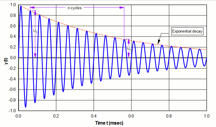
说明:
- 振幅 \( U_0 \) 和 \( U_n \) 可以采用任何一致的类型(峰值或峰‑峰值)。为方便起见,上图使用峰值振幅。
- 可以选择任意一个振荡峰值来测量 \( U_0 \)。
- \( n \) 是任意的。不过,较大的 \( n \) 会提高计算精度。
- 随着 \( U_0 \) 与 \( U_n \) 之间的差值变小(即振幅衰减得更慢),\( \delta \) 也变得更小。
对于图 1 所示的例子,对数衰减率为 —
\begin{align} \label{eq:13403a} \delta &= (1/10) \ln \left[ \frac{0.889}{0.346} \right] \\[0.7em]%eqn_interline_spacing &= 0.094 \nonumber \end{align}
注:图 1 显示 \( t = 0 \) 时起始振幅为 0,但这是任意的。计算得到的 \( \delta \) 不取决于起始振幅。可以想象将整个振幅波形向左或向右平移,便可看出这一点。
与 Q 的关系
\( \delta \) 与 Q(品质因数)的关系为 —
\begin{align} \label{eq:13404a} Q = \frac{\pi}{\delta} \end{align}
因此,当 \( \delta \) 很小(振幅衰减缓慢)时,\( Q \) 很大。
Log decrement (δ)
When a system is caused to oscillate and is then released from any external forcing functions (i.e., the system is then in free vibration), the amplitude decays because of loss within the system. The decay is exponential as given by the equation —
\begin{align} \label{eq:13401a} u = U e^{-(\delta \, f \, t)} \sin(2\pi \, f \, t) \end{align}
where —
| \( u \) | = instantaneous amplitude |
| \( U \) | = some peak amplitude |
| \( \delta \) | = log decrement |
| \( f \) | = frequency |
| \( t \) | = time |
(The exponent in equation \eqref{eq:13401a} is actually approximate but is nearly exact when \( \delta ≤ 2 \), which is appropriate for all ultrasonic systems.)
An example of equation \eqref{eq:13401a} is shown as the dotted line in figure 1. Note that larger values of \( \delta \) will cause the amplitude to decay more rapidly.
From equation \eqref{eq:13401a} it can be shown that if an amplitude maximum is measured at time \( t_0 \) and again later at time \( t_n \), the log decrement is given by (see figure 1) —
\begin{align} \label{eq:13402a} \delta = (1/n) \ln \left[ \frac{U_0}{U_n} \right] \end{align}
where —
| \( U_0 \) | = amplitude at time \( t_0 \) |
| \( U_n \) | = amplitude after \( n \) subsequent cycles |
| \( n \) | = number of cycles between \( U_0 \) and \( U_n \) |
|
|
|
Notes:
- The amplitudes \( U_0 \) and \( U_n \) can be any consistent type (peak or peak‑to‑peak). The above graph uses peak amplitudes for convenience.
- Any oscillation peak can be chosen to measure \( U_0 \).
- \( n \) is arbitrary. However, a large \( n \) will increase the calculation accuracy.
- As the difference between \( U_0 \) and \( U_n \) becomes smaller (i.e., a more slowly decaying amplitude), \( \delta \) also becomes smaller.
For the example of figure 1 the log decrement is —
\begin{align} \label{eq:13403a} \delta &= (1/10) \ln \left[ \frac{0.889}{0.346} \right] \\[0.7em]%eqn_interline_spacing &= 0.094 \nonumber \end{align}
Note: Figure 1 shows a starting amplitude of 0 at \( t = 0 \) but this is arbitrary. The calculated \( \delta \) does not depend on the starting amplitude. This can be seen by imagining the entire amplitude waveform being shifted left or right.
Relation to Q
\( \delta \) and Q (quality factor) are related by —
\begin{align} \label{eq:13404a} Q = \frac{\pi}{\delta} \end{align}
Thus, when \( \delta \) is small (a slowly decaying amplitude) \( Q \) is large.
Also see —
Attenuation
Bandwidth
Damping ratio
Loss tangent